Steam power: enthalpy, state evidence and efficiency boundaries

By How things work · myAudience

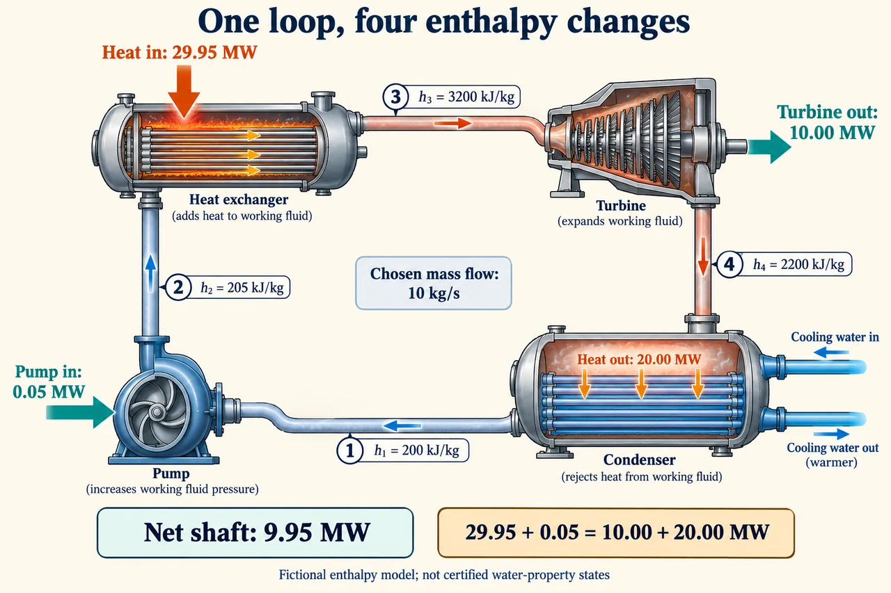
myAudience original rendered teaching illustration. Image: illustration, not a documentary photograph. · Operator-authored generated illustration; independent scientific acceptance pending.

Steam power: enthalpy, state evidence and efficiency boundaries

A steam cycle is a repeated route for a working fluid, but the fluid crosses the inlet and outlet of each component. That distinction lets us keep a closed-loop inventory while analysing an individual turbine as a steady-flow control volume. For one inlet and one outlet, heat supplied minus shaft work delivered equals mass flow multiplied by the change in enthalpy, kinetic energy and gravitational potential energy, provided stored energy is not changing. Use one declared sign convention throughout. The plate traces pump → heat addition → turbine → condenser → pump, with state numbers attached to that route. Its separate blue cooling circuit carries energy away through a solid wall; it is not mixed into the working-fluid loop. This is an accounting schematic, not a working construction drawing.

Enthalpy per unit mass is h = u + pv: internal energy u plus the pressure-volume term associated with moving fluid across a control boundary. In SI units, kPa multiplied by m³/kg gives kJ/kg. A turbine calculation based only on a temperature drop can miss phase change and pressure-dependent properties; a constant heat-capacity approximation is not a general steam-property model. Enthalpy references are conventional, so common-reference differences determine these balances, not an absolute claim that a state contains zero energy. The historical DOE fundamentals handbook explains these definitions. IAPWS's revised industrial formulation provides a defined state-property framework; real pressure, temperature, phase and validity-region evidence are needed before using it, rather than treating any chosen list of enthalpies as a feasible steam cycle.

Choose a fictional steady mass flow of 10 kg/s and the plate's h1 = 200, h2 = 205, h3 = 3,200 and h4 = 2,200 kJ/kg. Here state 1 is condenser outlet, 2 pump outlet, 3 turbine inlet and 4 turbine outlet. For this exercise, heat exchange in the pump and turbine, external loop losses and kinetic and potential energy differences are omitted. Pump input is 10(205 − 200) = 50 kW. Heat supplied to the working fluid is 10(3,200 − 205) = 29,950 kW. Turbine shaft output is 10(3,200 − 2,200) = 10,000 kW. Condenser rejection is 10(2,200 − 200) = 20,000 kW. These four numbers explain the plate's 0.05, 29.95, 10 and 20 MW boxes, with heat and shaft arrows serving different transfers.

Net shaft output subtracts the pump input once: 10,000 − 50 = 9,950 kW. The cycle balance is 29,950 + 50 = 10,000 + 20,000 kW, or equivalently 29,950 = 9,950 + 20,000. Net shaft efficiency relative to heat supplied to the fluid is 9,950/29,950 = 33.222…%. It is not exported electrical efficiency relative to fuel: combustion or other upstream heat delivery, generator conversion and other auxiliary loads are outside this selected boundary. Calling the 10 MW turbine output net, subtracting the same pump twice, or adding condenser rejection to electricity without a heat user would each change the definition. A balanced arithmetic table is necessary evidence, but it cannot by itself establish valid pressures, phases, entropy changes or a practical turbine.

Component efficiency answers a different question. Suppose a separate chosen turbine comparison uses the same inlet and exhaust pressure, with an isentropic outlet enthalpy h4s = 2,000 kJ/kg and actual outlet 2,200. Then turbine isentropic efficiency is (3,200 − 2,200)/(3,200 − 2,000) = 5/6, about 83.33%, not the cycle's 33.22%. The isentropic reference is a reversible adiabatic comparison, not an instruction to impose a real outlet state. Its physical consistency still requires state-property evidence. If only actual h4 rises to 2,300 in our accounting exercise, turbine output falls to 9 MW, net output to 8.95 MW and rejection rises to 21 MW. Heat input stays 29.95 MW under those explicit fixed-state assumptions, so net efficiency becomes 29.883…%. That change redistributes the same input rather than destroying energy.

A Carnot bound is about a reversible engine exchanging heat with two ideal reservoirs at constant absolute temperatures. For a separate 600 K hot reservoir and 300 K cold reservoir, the maximum fraction is 1 − 300/600 = 0.50. Irreversibility reduces the attainable conversion, but the 33.22% table does not prove a physically feasible steam path merely by lying below 50%. A steam inlet temperature is not automatically the temperature of an entire heat-supply reservoir: heat can be added across varying fluid temperatures. Celsius ratios are invalid because their zero is not absolute zero. A cyclic working fluid returns to its original entropy; irreversible operation increases the total entropy of the complete fluid-plus-environment accounting. Confusing those boundaries can make a first-law-correct story violate the second law.

A transfer calculation tests what was omitted. If an inlet speed is 20 m/s and an outlet speed 100 m/s, the outlet kinetic-energy rise is (100² − 20²)/2 = 4,800 J/kg = 4.8 kJ/kg. At the chosen 10 kg/s this is 48 kW. For the same enthalpy drop in an adiabatic turbine with unchanged elevation, shaft output is 10,000 − 48 = 9,952 kW, so net output after the 50 kW pump is 9,902 kW. Leaving the outlet jet outside the selected loop means it carries 48 kW across that boundary; a later diffuser or dissipative recovery must be modelled explicitly before asserting the original condenser balance. Doubling mass flow would double powers only if these states and losses stayed fixed, an assumption actual equipment may not satisfy.

Numerical precision is not measurement certainty. Flow and state errors propagate into a difference of enthalpies; near-cancelling terms can make relative uncertainty large. Compare alternatives delivering the same needed electrical and thermal services, with the same fuel convention, upstream boundary and auxiliary accounting. Maintenance, water use, embodied equipment and local receiving-water effects require separate evidence; no conversion percentage alone establishes a fair or low-impact project. Ask who receives reliable service, who bears outage and thermal burdens, and whether reported gains exceed uncertainty. Report the dated handbook as a fundamentals source, not a current plant performance promise. The plate's entries are deliberately chosen educational numbers, not operating limits or verified water-property states. Image: illustration, not a documentary photograph.

Worked example: Use the chosen four-state table at 10 kg/s. Compute each component transfer, net shaft efficiency and the revised result if only h4 changes to 2,300 kJ/kg. Explain why neither result establishes electrical fuel efficiency.

Pump input = 10(205 − 200) = 50 kW; heat into the working fluid = 10(3,200 − 205) = 29,950 kW.

Initial turbine output = 10,000 kW and condenser rejection = 20,000 kW; 29,950 + 50 = 10,000 + 20,000.

Initial net = 9,950 kW; 9,950/29,950 = 0.3322203673.

With h4 = 2,300, turbine = 9,000, rejection = 21,000 and net = 8,950 kW; 8,950/29,950 = 0.2988313856.

The denominators are heat delivered to the working fluid, not fuel input. Generator losses and other auxiliary loads remain outside this model.

Answer: Initial net 9.95 MW at 33.222…%; changed net 8.95 MW at 29.883…%. Both balances close. Neither certifies a physical state path or exported electrical fuel efficiency.

Check your understanding: An advertiser claims 65% conversion between two ideal reservoirs at 450°C and 30°C. Is that compatible with their stated boundary? Separately, what shaft correction follows from the 20 to 100 m/s speed change?

Answer: Convert to 723.15 K and 303.15 K: the reversible bound is 1 − 303.15/723.15 = 58.079…%, so 65% is incompatible if those truly are the only two constant-temperature reservoirs and no other energy input exists. A change of boundary could explain a different metric, not rescue this claim. The kinetic-energy rise is 4.8 kJ/kg, taking 48 kW from shaft output at 10 kg/s; turbine 9,952 and net 9,902 kW.

Why: Use absolute temperatures and the complete stated energy boundary. Enthalpy drop is not all shaft work when outlet kinetic energy increases.