Steam power: condenser resistance and useful heat over time

By How things work · myAudience

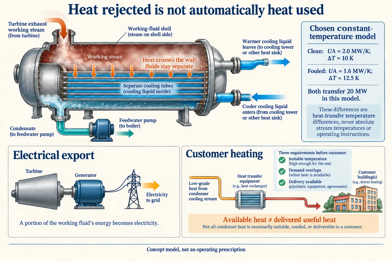
myAudience original rendered teaching illustration. Image: illustration, not a documentary photograph. · Operator-authored generated illustration; independent scientific acceptance pending.

Steam power: condenser resistance and useful heat over time

A surface condenser is an interface between two distinct circuits. Steam on one side releases energy and forms condensate; cooling fluid on the other absorbs energy through the separating tube wall. The plate's steam inlet and condensate outlet belong to the working-fluid loop, while the blue inlet and warmer outlet belong to the cooling circuit. The feed pump returns working-fluid condensate, not cooling water. Condensation helps establish the turbine's exhaust condition; changing that condition can change work extracted, but the relationship depends on a complete valid cycle and equipment constraints. Cooling fluid is a heat sink for this transfer. An available heat sink is not automatically a useful customer heat service, and a conceptual cutaway cannot specify a safe plant design.

Heat-transfer conductance UA combines area with an overall coefficient covering the fluid films and solid wall. Write heat rate Qdot = UA × ΔTeffective for a stated heat-exchanger model. The plate deliberately chooses an ideal constant-temperature comparison: UA = 2 MW/K and a 10 K difference transfer 20 MW. If added resistance reduces UA to 1.6 MW/K, the same 20 MW would require 12.5 K; at an unchanged 10 K it transfers only 16 MW. These are conditional alternatives, not simultaneous descriptions of one steady unchanged plant. The drawn cooling outlet is warmer than its inlet, so a real finite-flow exchanger would need a varying-temperature analysis, often a log-mean temperature difference with appropriate configuration assumptions. Do not substitute its inlet difference for the effective difference without justification.

In the lumped comparison, resistance is 1/UA. Clean resistance is 0.5 K/MW and the changed resistance is 0.625 K/MW, an increase of 0.125 K/MW. This explains why a lower conductance can require a larger driving difference; it does not identify whether a particular deposit, fluid film or tube caused the change. The dated DOE survey discusses condenser performance effects including fouling, noncondensable gases and cooling conditions. A diagnosis needs measurements and competing explanations, not a single performance ratio. If 20 MW enters while only 16 MW leaves, 4 MW must accumulate or another transfer/state must change; declaring steady state while silently discarding that difference violates conservation. These lessons explain mechanisms, not cleaning, pressure or maintenance procedures.

The plate's heat-user branch is a decision schematic. Rejected energy must be at a suitable temperature for the service, available when demand exists, and delivered through appropriate equipment. A passive exchanger cannot raise the receiving stream above the supplying stream's available temperature; upgrading low-temperature heat may require a heat pump and additional electrical accounting. A symbol for a customer does not supply a completed delivery-and-return circuit. Counting all condenser heat as useful merely because it leaves a plant overstates service. EPA's total-system accounting adds net electrical and useful thermal outputs over the same fuel input; it also notes that this sum does not give electricity and heat the same practical value. Keep separate service quantities visible alongside the combined percentage.

Choose a separate fictional 1,000-hour planning window, unrelated to any real plant: gross electrical output while operating is 10 MW, electrical auxiliaries 0.5 MW and fuel input 33 MW on one consistently chosen heating-value basis. Availability is 0.90, giving 900 operating hours. Assume constant on-state powers, no start-up or standby fuel, and no exported heat pumping or delivery losses for this exercise. Expected net electricity is (10 − 0.5) × 900 = 8,550 MWh; fuel input is 33 × 900 = 29,700 MWh. This fuel boundary differs from the previous lesson's 29.95 MW heat delivered to its working fluid. The numbers must not be spliced together to imply a measured boiler efficiency or a certified feasible state path.

Assume suitable-temperature heat could be supplied at 12 MW while operating, but the customer's demand is capped at 8 MW during exactly 500 scheduled hours and zero otherwise. Under the additional chosen assumption that operating availability is independent of the demand schedule, expected coincident operating hours are 0.90 × 500 = 450, so useful heat is 8 × 450 = 3,600 MWh. The 12 MW potential does not override the 8 MW service cap. Combined service fraction is (8,550 + 3,600)/29,700 = 40.909…%, while exported electrical fraction alone is 8,550/29,700 = 28.787…%. These two numbers answer different questions. Neither includes a comparison with displaced generation or heating, and neither alone proves a reduction in costs, emissions or community burdens.

Availability by itself does not determine useful heat. Retain exactly 900 operating hours in the same 1,000-hour window: there are 100 outage hours. If all outages coincide with the customer's 500 demand hours, only 400 demand hours are served and useful heat is 3,200 MWh. If all outages occur outside demand, all 500 demand hours are served and heat is 4,000 MWh. Thus the feasible range under this schedule is 3,200–4,000 MWh; independence gave an expectation of 3,600, not a guaranteed result. With the same 8,550 MWh electricity and 29,700 MWh fuel, combined fractions range from 39.562…% to 42.255…%. A planned maintenance timetable can therefore change service without changing the headline annual availability. Correlated demand, start-up constraints or variable output require a richer model.

Evaluate a maintenance proposal using equivalent services and explicit trade-offs. Better availability can increase delivered electricity but also increase total fuel burned; a larger energy sum is not automatically less environmental impact. A useful-heat claim should identify temperature evidence, customer coincidence, delivery losses and the displaced alternative before claiming benefits. Materials, cooling-water withdrawal, receiving-water temperature, workforce protection and accessible outage information belong in the decision even though this arithmetic assigns them no price. Examine who loses heat during an outage and whether redundancy or scheduling can protect vulnerable users. The plate distinguishes heat rejection from usable service and marks its UA comparison as an ideal teaching model; it supplies no clinical, construction or plant operating limits. Image: illustration, not a documentary photograph.

Worked example: For the declared 1,000-hour fictional service model, derive the independent-availability expected useful heat and then rigorous coincidence bounds given exactly 100 outage hours. Keep fuel and net electricity identical between these schedule cases.

Operating time = 0.90 × 1,000 = 900 h. Net electricity = 9.5 × 900 = 8,550 MWh; fuel = 33 × 900 = 29,700 MWh.

Independent expected overlap = 0.90 × 500 = 450 h. Demand-limited heat = min(12,8) × 450 = 3,600 MWh.

Maximum overlap is 500 h if the 100 outage hours are outside demand; minimum is 500 − 100 = 400 h if they all coincide. Heat bounds are 4,000 and 3,200 MWh.

Combined fractions: expected 12,150/29,700 = 40.909…%; lower 11,750/29,700 = 39.562…%; upper 12,550/29,700 = 42.255…%.

These bounds rely on the chosen fixed powers, adequate heat temperature and zero delivery/start-up losses; annual availability alone cannot choose a value within them.

Answer: Expected useful heat 3,600 MWh only under independence. Fixed-uptime bounds are 3,200–4,000 MWh, despite identical 8,550 MWh net electricity. Report the schedule assumption, not a guaranteed 40.909…% service fraction.

Check your understanding: UA falls from 2 to 1.6 MW/K. Someone keeps both heat transfer 20 MW and effective temperature difference 10 K, then counts 12 MW potential customer heat throughout all 900 operating hours. Identify and quantify both errors.

Answer: At 10 K the changed exchanger model transfers 16 MW, not 20; retaining 20 needs 12.5 K or changed model evidence. A claimed steady 20-in/16-out balance has an unexplained 4 MW. Potential customer heat 12 × 900 = 10,800 MWh ignores the 8 MW demand cap and 500-hour schedule; independent expected useful heat is 3,600 MWh, so that claim overstates it by 7,200 MWh. The heat amount also requires suitable temperature and delivery evidence.

Why: Separate heat-transfer capacity from a steady balance, and potential heat from service actually demanded and delivered over coincident hours.