Growth, cost models and the limits of efficiency

By UK A Level Computer Science · independent study · myAudience

Original textbook concept plate generated with OpenAI imagegen; labels and states checked against the lesson model. · Generated original teaching artwork; pending operator rights/provenance review before publication.

Growth, cost models and the limits of efficiency

Algorithm analysis begins by defining input size and a counted operation. For a list search, n can be the number of elements and the operation a key comparison. For multiplication of arbitrarily large integers, input size is more naturally the number of bits. A function maps a domain to values in a codomain; a cost function T(n) maps allowed sizes to a nonnegative operation count. The same program may have different best, worst and expected counts. State which one is analysed before assigning a complexity class.

Big-O is an asymptotic upper bound: T(n) is O(g(n)) when constants c>0 and n₀ exist such that T(n)≤c g(n) for all allowed n≥n₀. Theta denotes a matching upper and lower order; little-o, not needed here, denotes a stricter asymptotic relation. If T(n)=3n²+2n+7, then for n≥1 it is at most 12n² and at least 3n², so T(n)=Θ(n²). It is also O(n³), but that looser upper bound hides useful information. Big-O does not literally mean worst case: a best-case cost function can also be bounded with it.

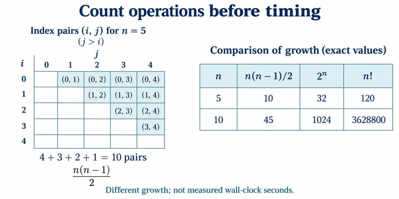
Our pair_count enumerates pairs of distinct indices with i<j. Its nested loops do not always perform n² operations: for i=0 the inner loop runs n−1 times, then n−2, down to zero. The exact count is n(n−1)/2, with Θ(n²) growth. The alternative closed formula needs a fixed number of arithmetic operations under a unit-cost model. When n itself is supplied in binary, that model hides the cost of arithmetic on growing operands and the impossibility of explicitly outputting all pairs in fewer than their number of output steps.

Repeated halving produces logarithmic growth: after k halvings a size n region is about n/2ᵏ, so k≈log₂n. A fixed number of passes produces linear growth, and nested independent n-step loops produce quadratic growth. Enumerating all subsets of n distinct items produces 2ⁿ possibilities; enumerating all permutations produces n!. For n=10, these counts are 1,024 and 3,628,800 respectively. Factorial is not the same as quadratic or simply “another polynomial”. Domain constraints can shrink a search space, but an optimisation needs evidence that it preserves required answers.

Polynomial-time solvability is the syllabus's tractability distinction. A known exponential brute-force algorithm does not prove that no polynomial algorithm exists. Conversely, polynomial time is not a guarantee of practical speed: n¹⁰ and enormous constants can be unusable. Heuristics may trade guaranteed optimality or completeness for useful answers, and those losses belong in the contract. A faster processor multiplies a feasible operation budget by a finite factor; it does not change an exponential growth function into a polynomial one. Empirical timings can test an implementation on selected inputs, while mathematical analysis supports a broader asymptotic claim under explicit assumptions.

Reading the diagram: The triangular grid includes a cell only when j>i, so there are 4+3+2+1=10 unordered index pairs for n=5. Blank cells are not zero-weight pairs; those pairs are excluded. The comparison table gives pair counts 10 and 45, subset counts 32 and 1024, and permutation counts 120 and 3628800 for n=5 and 10. These are exact combinatorial counts, not measured elapsed times. Different output families cannot be compared as though they solved the same required task.

Runnable original Python 3, independently executed on Python the related topic. Read the stated input contract before running. These examples use fictional data and are teaching models, not production services.

```python
def pair_count(n):
"""Count unordered index pairs explicitly, not by the closed formula."""
count = 0
for i in range(n):
for j in range(i + 1, n):
count += 1
return count
```

Worked example: Derive pair_count(5) and compare its exact work with doubling input size.

For i=0,1,2,3,4 the inner counts are 4,3,2,1,0, totalling 10.

The closed form gives 5×4/2=10, establishing agreement on this instance.

At n=10 there are 45 pairs, not exactly four times 10. The ratio approaches four as n grows because the leading quadratic term dominates the linear correction.

Answer: 10 pairs at n=5 and 45 at n=10; asymptotic quadratic growth does not assert exact finite-size ratios.

Check your understanding: 1. Give pair counts for n=0 and n=1. 2. Bound 3n²+2n+7 by a constant times n² for n≥1. 3. A search doubles work whenever n increases by one. What can a processor 1,024 times faster buy, and what can it not establish?

Answer: 1. Both are zero because no distinct index pair exists. 2. Since 2n≤2n² and 7≤7n², the total is at most 12n², with a lower bound 3n². 3. A 1,024=2¹⁰ speed factor buys roughly ten additional units of n at the same budget for a pure 2ⁿ cost. It does not establish polynomial scalability or prove that the underlying problem has no better algorithm.

Why: Count actual loop ranges. Do not read Big-O as an exact stopwatch time or automatic worst-case label. Hardware factors do not change asymptotic class. A slow known algorithm is evidence about that algorithm, not a proof of intrinsic intractability.