Gas turbines: internal work, irreversibility and the limits of optimisation

By How things work · myAudience

myAudience original rendered teaching illustration. Image: illustration, not a documentary photograph. · Operator-authored generated illustration; scientific model reviewed separately.

Gas turbines: internal work, irreversibility and the limits of optimisation

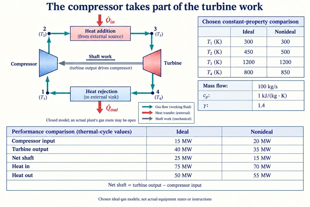
A turbine can produce substantial shaft work while exporting much less, because its compressor consumes part of that work. The plate's grey arrow therefore points from the turbine toward the compressor; it is a mechanical transfer, not the coloured gas route. A real combustion gas turbine takes in air and discharges exhaust. Here, deliberately use a closed thermodynamic surrogate that heats and cools the same ideal-gas mass without fuel addition. The four numbered states are accounting states rather than real combustor settings. Choose a constant mass flow of 100 kg/s, constant cp = 1 kJ/(kg K) and γ = 1.4. These stipulated properties are not measured air properties valid over every depicted temperature.

Trace 1 → 2 compression, 2 → 3 external heat addition, 3 → 4 expansion and 4 → 1 external heat rejection. Neglect kinetic and potential energy changes, pressure losses in the heaters and any heat transfer in compressor or turbine. The ideal comparison additionally requires reversible compression and expansion. Adiabatic alone does not establish an isentropic process: friction can generate entropy without external heat. For the ideal gas and these constant properties, define x = rp^((γ − 1)/γ), where rp is the compressor pressure ratio. Then T2/T1 = x and T3/T4 = x. Temperatures in these ratios must be absolute kelvins. NASA's educational compressor and Brayton descriptions support the ideal relationships; their aircraft thrust examples are not stationary-generator export accounts.

The left table's ideal states are T1 = 300 K, T2 = 450 K, T3 = 1200 K and T4 = 800 K. Both temperature ratios give x = 1.5, so rp = 1.5^3.5 ≈ 4.1335. Specific compressor input is cp(T2 − T1) = 150 kJ/kg; turbine output is cp(T3 − T4) = 400 kJ/kg. Multiplying by 100 kg/s gives 15 MW input and 40 MW output, leaving 25 MW net shaft work. Heat addition is 75 MW and rejection is 50 MW, satisfying 75 = 25 + 50. Back-work ratio is 15/40 = 37.5%, whereas cycle thermal efficiency is 25/75 = 33.33…%. These distinct ratios answer different questions; net shaft output still needs generator and plant-auxiliary boundaries before claiming electrical export or fuel efficiency.

The right table keeps the same stipulated pressure ratio, T1 and T3, but chooses irreversible adiabatic component outcomes T2 = 500 K and T4 = 850 K. Compressor input becomes 20 MW, turbine output 35 MW and net shaft work 15 MW. Heat addition is now 70 MW, not the ideal table's 75 MW; rejection is 55 MW, closing 70 = 15 + 55. Back-work ratio rises to 20/35 ≈ 57.14%, while efficiency falls to 15/70 ≈ 21.43%. Increasing compressor temperature costs input work; increasing turbine exit temperature leaves less expansion work. Using an unchanged ideal heat-input denominator would mix two different state models and hide an accounting error rather than describe a component improvement.

Component efficiencies compare an actual outcome with its reversible counterpart at the same relevant inlet state and pressure change. Here ηc = (450 − 300)/(500 − 300) = 0.75, and ηt = (1200 − 850)/(1200 − 800) = 0.875. Adding or averaging them does not yield whole-cycle efficiency. A constant-property entropy check is also possible: relative to the ideal endpoint at the same pressure, the chosen compressor entropy increase is cp ln(500/450) ≈ 0.10536 kJ/(kg K), and the turbine increase is cp ln(850/800) ≈ 0.06062 kJ/(kg K). Both are positive, consistent with the stipulated adiabatic irreversibility. An apparent negative value would require revisiting the boundary and assumptions; it would not be evidence that losses mysteriously improved performance.

Optimisation needs a declared objective. For ideal components with fixed T1 and T3, specific net work is wn = cp[T3(1 − 1/x) − T1(x − 1)]. Differentiate with respect to x: dwn/dx = cp(T3/x² − T1), so the maximum occurs at x = √(T3/T1) = 2 in this model. The second derivative is −2cpT3/x³, negative for x > 0. At that point T2 = T4 = 600 K, compressor input is 300 kJ/kg, turbine output 600 kJ/kg and net work 300 kJ/kg, or 30 MW at the chosen flow. Heat addition is 60 MW and efficiency 50%. This is a mathematical optimum of a deliberately limited surrogate, not a recommended pressure or temperature for an installation.

Efficiency alone points toward a different direction: the ideal formula η = 1 − 1/x increases with x. Positive heat addition and positive net work require 1 < x < T3/T1 = 4. As x approaches 4, both heat addition and net output approach zero. The limiting efficiency is 75%, but at x = 4 the direct ratio is 0/0 and there is no finite-power engine output to celebrate. If a separate stipulated constraint restricts x to at most 1.8, the positive derivative below 2 makes x = 1.8 the constrained net-work maximum: 293.333… kJ/kg, or 29.333… MW. Show the constraint and evaluate the objective rather than apply an unconstrained optimum automatically. The worked example and check test these different decisions.

A real assessment must restore variable gas properties, combustion and fuel energy, pressure losses, cooling and material limits, emissions and auxiliary demands. NASA's turbine explanation identifies material and cooling challenges; DOE describes compressor demand and exhaust recovery. Their historical performance numbers are not guarantees adopted here. Efficiency can lower fuel use for a fixed delivered service while still leaving lifecycle fuel and pollution burdens, unequal local exposures and maintenance costs. Ask who receives reliable service, who lives near emissions sources, and who can verify the evidence. The plate is a bounded cycle model with explicit state and work bookkeeping; it cannot establish equipment compatibility, safe operation or a complete lifecycle comparison. Image: illustration, not a documentary photograph.

Worked example: Using the declared constant-property surrogate, calculate ideal and nonideal net work, heat input, back-work ratio and efficiency. Then find the ideal pressure-ratio factor x that maximises net work for T1 = 300 K and T3 = 1200 K, including the constrained case x ≤ 1.8.

Ideal: compressor = 100 × 1 × 150 = 15,000 kW; turbine = 40,000 kW; net = 25 MW. Heat input = 75 MW and rejection = 50 MW. Back-work ratio = 0.375; efficiency = 25/75 = 1/3.

Nonideal: compressor = 20 MW; turbine = 35 MW; net = 15 MW. Heat input = 70 MW; rejection = 55 MW. Back-work ratio = 4/7; efficiency = 3/14.

Set cp(T3/x² − T1) = 0: x = 2. Then rp = 2^3.5 ≈ 11.3137, T2 = T4 = 600 K, and net specific work = 300 kJ/kg, giving 30 MW at 100 kg/s.

With 1 < x ≤ 1.8, net work increases throughout that interval, so use x = 1.8. Specific net work = 1200(1 − 1/1.8) − 300(1.8 − 1) = 293.333… kJ/kg; power = 29.333… MW.

Answer: Ideal: 25 MW net, 75 MW input, 37.5% back work and 33.33…% efficiency. Nonideal: 15 MW net, 70 MW input, 57.14…% back work and 21.43…% efficiency. The model-only net-work maximum is 30 MW at x = 2; the constrained maximum is 29.333… MW at x = 1.8.

Check your understanding: A comparison claims that ηc + ηt = 162.5% proves an excellent plant and that choosing x = 4 gives 75% efficiency at useful output. Correct both claims. Explain why a fixed gas mass-flow comparison is different from comparing equal delivered electricity.

Answer: The component ratios use different ideal reference work transfers and cannot be added as a whole-cycle efficiency. For the chosen nonideal states, net shaft work divided by heat input is 15/70 ≈ 21.43%; actual fuel-to-electricity efficiency needs further boundaries. At x = 4, T2 = T3 and T4 = T1: both heat input and net work vanish, so the exact efficiency ratio is undefined. A 75% limiting ratio is not finite output. Fixed mass flow holds one input to the thermodynamic calculation constant; equal delivered electricity may require different flow, fuel, auxiliaries or availability. A fair service comparison must specify those quantities and constraints before assigning cost or environmental benefits.

Why: Keep reference ratios separate, test boundary cases and constraints, and distinguish a mathematical limit from useful service under a complete energy boundary.