Solar receivers: why a hotter cycle need not yield more electricity

By How things work · myAudience

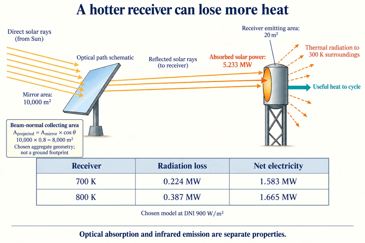
Image: illustration, not a documentary photograph. · Operator-authored generated illustration; scientific model reviewed separately.

Solar receivers: why a hotter cycle need not yield more electricity

Concentrating solar thermal equipment collects direct sunlight as heat before a separate heat engine produces electricity. The existing lesson traces the storage and working-fluid loops. Here the question is more demanding: if a hotter heat engine converts a larger fraction of its heat input to work, must a hotter receiver also export more electricity? A receiver loses heat, and the field has optical losses before any energy reaches the working fluid. Define the comparison across sunlight entering the mirror field and net electricity leaving the chosen plant boundary. Compare both designs under the same incident resource, mirror assumptions and auxiliary account. A cycle-only efficiency cannot decide the field-to-grid outcome.

Direct normal irradiance, DNI, measures direct-beam power per area perpendicular to the beam. Diffuse sunlight arrives from many directions; replacing DNI with global irradiance would assume that all those directions can be focused by the same mirror geometry. Define θ between the mirror normal and the incoming beam; the plate’s separate area card expresses an aggregate cosine model, not a geometric ground footprint. The chosen aggregate cosine is 0.8, so 10,000 m² of mirror area intercepts the beam as 8,000 m² of projected area. Multiplication by a chosen reflectance 0.9, receiver-interception fraction 0.85 and solar absorptance 0.95 gives the absorbed power. These factors describe different destinations: reflected elsewhere, missing the receiver, or arriving but not being absorbed. Concentration redirects collected power; it never multiplies the energy originally intercepted. A real field needs a geometry-dependent model rather than one representative cosine.

For the invented clear-resource case, DNI is 900 W/m². Absorbed power is 900 × 10,000 × 0.8 × 0.9 × 0.85 × 0.95 = 5,232,600 W, or 5.2326 MW. The receiver's emitting surface is a separate chosen 20 m², not the mirror field's 10,000 m². The drawing uses distinct labels for these areas because swapping them would change radiation loss by a factor of 500. Follow the orange input arrow into the receiver and the outgoing radiative arrows toward the surroundings; follow the teal useful-heat arrow toward the cycle. Neither the incoming sunlight nor an outgoing heat-loss arrow is an electrical output. The plate rounds 5.2326 to 5.233 MW for legibility, while the calculation retains the unrounded value.

Model the receiver as a uniform-temperature surface exchanging long-wave radiation with large uniform 300 K surroundings, with view factor one and constant effective infrared emissivity 0.85. Its positive outward loss is ε σ A_receiver(T⁴ − T_surroundings⁴), using σ = 5.67 × 10⁻⁸ W/(m² K⁴). Temperatures must be in kelvin: a fourth power of degrees Celsius does not express this law. At 700 K the loss is 0.2236248 MW; at 800 K it is 0.38700585 MW. Optical solar absorptance and infrared emissivity refer to different spectral ranges, so the chosen 0.95 and 0.85 are not contradictory or automatically interchangeable. A real receiver has nonuniform flux, geometry and surface properties; this single-surface law is a bounded teaching surrogate, not a validated receiver design.

Add a stipulated constant 0.2 MW of other receiver thermal losses and assume steady state, with no energy accumulating in the receiver. Useful heat is therefore absorbed solar power minus radiation and those other losses. Choose gross cycle conversion of 0.35 in the 700 K case and 0.38 in the 800 K case, then subtract 0.1 MW of total electrical auxiliaries. The net exports are (5.2326 − 0.2236248 − 0.2) × 0.35 − 0.1 = 1.58314132 MW and (5.2326 − 0.38700585 − 0.2) × 0.38 − 0.1 = 1.665325777 MW. The plate's table rounds radiation and net electricity to three decimals. The hotter case wins by about 0.08218 MW under these chosen assumptions: its conversion gain more than compensates for its additional radiative loss. This is a conditional comparison, not proof that temperature alone caused a real installation's output.

Reduce DNI while holding every stipulated loss and conversion factor fixed to isolate the logical tradeoff. At 450 W/m², absorbed power halves to 2.6163 MW and net exports become 0.66743632 and 0.671131777 MW: the hotter case's advantage almost disappears. At 300 W/m², absorbed power is 1.7442 MW and exports become 0.36220132 and 0.339733777 MW. Now the cooler case wins because the larger receiver loss is paid from a smaller collected input. The algebra demonstrates a possible ranking reversal. It does not establish that an actual receiver can stay at either temperature at those irradiances, or that its real heat engine retains the same part-load conversion. Testing that physical feasibility is a different, necessary task.

Maintenance and materials affect the model terms rather than constituting one generic reliability allowance. Dirt on mirrors can change reflected and intercepted power; coating degradation can alter solar absorptance or infrared emissivity; wind and local surface temperatures can change nonradiative loss. Thermal cycling, corrosion and exchanger performance constrain useful service, while inspection and repair affect availability and cost. Evidence should separate measured optical performance, receiver heat balance, part-load cycle output and auxiliary demand across comparable conditions. A better model would include uncertainty and covariation instead of independently changing one convenient number. These distinctions are reasons to seek tested material and site data; they are not optical alignment, temperature-setting or hot-fluid handling instructions.

I would choose neither a hotter receiver nor a larger mirror field from a cycle percentage alone. A defensible comparison specifies the electricity service, weather distribution, maintainable materials and whole-system energy account, then tests whether the proposed advantage survives uncertain losses and realistic operating constraints. Cooling-water demand, habitat and land use, local maintenance employment, grid access and the allocation of project risks belong in the decision alongside output. A lower-temperature option can be preferable if it delivers adequate service with fewer material or maintenance burdens, while a hotter option needs evidence that additional useful conversion exceeds its losses over relevant conditions. The model supplies a mechanism and a testable comparison, not a universal project recommendation. Image: illustration, not a documentary photograph.

Worked example: Use the declared optical and receiver model at DNI 300 W/m². Compare 700 K/0.35 and 800 K/0.38 net exports, then explain why using mirror area in radiation or global irradiance as DNI would invalidate the comparison.

Absorbed direct power = 300 × 10,000 × 0.8 × 0.9 × 0.85 × 0.95 = 1.7442 MW. Use 20 m² emitting area, not 10,000 m² mirror area.

Positive outward radiative losses remain 0.2236248 MW at 700 K and 0.38700585 MW at 800 K under the uniform 300 K surroundings assumption.

Net 700 K = (1.7442 − 0.2236248 − 0.2) × 0.35 − 0.1 = 0.36220132 MW. Net 800 K = (1.7442 − 0.38700585 − 0.2) × 0.38 − 0.1 = 0.339733777 MW.

The hotter case loses by 0.022467543 MW. Larger radiative loss outweighs the chosen conversion gain here; the loss-area or irradiance substitutions change the physical boundary rather than improve the design.

Answer: The cooler case exports about 0.362 MW and the hotter case 0.340 MW in this chosen surrogate. Radiation depends on receiver emitting area and absolute temperature. DNI represents focusable direct-beam input; global radiation additionally includes diffuse directions. Actual feasibility, temperature distribution and part-load behaviour require independent evidence.

Check your understanding: Keep all model terms fixed except DNI. Derive the absorbed-power value at which the two net exports tie, then its corresponding DNI. Explain why this is not a real plant switching threshold.

Answer: Let P be absorbed power in MW, L₇₀₀ = 0.2236248 MW and L₈₀₀ = 0.38700585 MW. Equality 0.35(P − L₇₀₀ − 0.2) − 0.1 = 0.38(P − L₈₀₀ − 0.2) − 0.1 gives 0.03P = 0.38L₈₀₀ − 0.35L₇₀₀ + 0.006. Thus P ≈ 2.4931181 MW, and DNI ≈ 428.8128827 W/m² because absorbed power in MW = DNI × 0.005814. This is the crossing of two stipulated linear-in-input models with fixed losses and conversions. Receiver temperatures, emissivity, convection, part-load conversion and auxiliaries can vary with input, so the result is neither an operating instruction nor an observed universal threshold.

Why: Evaluate the complete input-to-export boundary and distinguish a mathematical crossing under chosen constants from measured plant behaviour.