Thermal storage: schedule useful service without counting energy twice

By How things work · myAudience

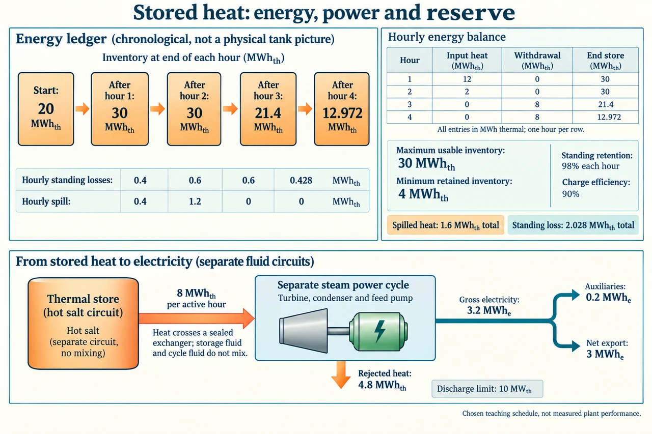
Image: illustration, not a documentary photograph. · Operator-authored generated illustration; scientific model reviewed separately.

Thermal storage: schedule useful service without counting energy twice

Thermal storage makes the timing of collection and electricity production partly separable, but dispatchable does not mean unlimited or guaranteed. The existing lesson converts a static sensible-heat inventory into a possible electrical total. This lesson follows chronological service: a store can have enough energy over a day yet fail a particular power request, spill collection when full, or need to retain inventory. Define a usable thermal-energy account relative to a chosen cooler reference, with a capacity of 30 MWh thermal and a retained reserve of 4 MWh thermal. These are invented accounting limits, not fluid freezing, pressure or equipment safety thresholds. Net electrical service lies across a separate power-cycle boundary, after auxiliaries.

Use four one-hour windows, initial inventory 20 MWh thermal and available collection heat 12, 2, 0 and 0 MWh thermal respectively. Charging retains 90% of that incoming heat in the usable store. Standing retention is 98% per window, applied to the inventory at the beginning of each window before any new charge or withdrawal. The simplified sequence chooses no simultaneous charging and dispatch: collection occurs in hours one and two, and electricity delivery in hours three and four. The plate's inventory arrows and table make this ordering visible. Changing the order changes when incoming energy can be lost or spilled, so it would define a different model rather than a harmless arithmetic rearrangement.

Before enforcing capacity, the balance is E_pre = 0.98 E_previous + 0.90 Q_in − Q_withdraw. End inventory is the smaller of E_pre and 30 MWh thermal, and any positive excess over 30 is recorded as spilled heat. A proposed withdrawal is feasible only if its resulting inventory stays at or above the 4 MWh thermal reserve and its one-hour quantity does not exceed a chosen 10 MW thermal discharge limit, equivalent here to 10 MWh thermal per window. Do not permit negative storage and subsequently claim the target was met. Do not silently erase spill. Reserving inventory protects the chosen future-service margin in this example; an actual installation also needs independently justified temperature, material and control limits.

The requested net electrical outputs are 0, 0, 3 and 3 MWh electrical. Choose 40% gross conversion from withdrawn heat to electricity, with 0.2 MWh electrical auxiliary demand in each active dispatch window only. Each active hour therefore requires (3 + 0.2)/0.40 = 8 MWh thermal. The lower plate treats the complete steam cycle as an energy-conversion boundary including turbine, condenser and feed pump. Its heat-input arrow represents transfer across a sealed exchanger: storage fluid and cycle water or steam do not mix. The chosen cycle rejects 8 − 3.2 = 4.8 MWh thermal per active hour. Its 3.2 MWh gross electrical arrow divides into 0.2 MWh of auxiliaries and 3 MWh exported. Counting the entire 3.2 as export would omit the auxiliary load; subtracting auxiliaries again from the thermal inventory would count them twice after the gross conversion account.

In hour one, standing loss removes 0.4 MWh thermal and charging contributes 10.8, giving 30.4 before capacity. Spill is 0.4 and end inventory is 30. Hour two loses 0.6, adds 1.8 and spills 1.2, ending again at 30. Hour three loses 0.6 and withdraws 8, ending at 21.4. Hour four loses 0.428 and withdraws 8, ending at 12.972. The total account closes: initial 20 + charged 12.6 − withdrawals 16 − spill 1.6 − standing loss 2.028 = final 12.972 MWh thermal. Gross electricity is 6.4 MWh, and subtracting 0.4 auxiliary demand leaves the requested 6 MWh export. The residual includes the 4 MWh reserve: only 8.972 is initially above it, before any later losses or further constraints.

A request for 5 MW net in a one-hour active window requires (5 + 0.2)/0.40 = 13 MW thermal under the same constant conversion and auxiliary assumptions. That exceeds the 10 MW thermal discharge limit even if the store holds ample energy. The largest conditional net output permitted by that power boundary is 10 × 0.40 − 0.2 = 3.8 MW. The constraint is power, not total inventory. In a separate low-inventory, no-collection scenario beginning with 6 MWh thermal, standing loss leaves 5.88. Keeping the 4 reserve permits only 1.88 withdrawal, giving 1.88 × 0.40 − 0.2 = 0.552 MWh net if that same active auxiliary demand applies. A 3 MWh request then has a 2.448 MWh shortfall. This second constraint is available energy, and real startup conditions could make even the partial dispatch infeasible.

A schedule should be evaluated against forecast errors and maintenance states, not only the sunny central case. Storage may shift heat use into an evening demand window, yet clouds can reduce charging before that window, and a full store can discard early collection that a later deficit would need. Real thermal stratification, heat-exchanger approach temperatures, cycle startup, ramps, part-load efficiency and cooling availability alter useful output. Two chosen scenarios do not give a probability of meeting service. Measurements, weather histories and validated component behaviour are needed before a reliability claim. DOE describes direct, indirect and thermocline architectures; this lumped energy ledger does not distinguish all their temperature distributions or certify the performance of any one of them.

I would first ask which service must be provided, at what times and with what acceptable shortfall, then compare feasible schedules and alternatives across energy, power, reserve and lifecycle boundaries. More storage capacity cannot alone solve an insufficient discharge-power limit; a higher-power cycle cannot create heat missing after clouds. Deliberate curtailment, changed demand timing or another supply may be preferable to an oversized project, depending on evidence. Cooling water, land and habitat impacts, maintainable components, affordable access and who bears unmet-service risks deserve explicit evaluation. The full chronological balance helps make those choices accountable, but it is not a plant operating procedure or a guaranteed reliability forecast. Image: illustration, not a documentary photograph.

Worked example: Recompute the four-hour schedule from 20 MWh thermal, showing standing loss, charge, spill, withdrawal and export separately. Verify global thermal conservation and retained reserve.

Hour 1: 20 × 0.98 + 12 × 0.9 = 30.4; spill 0.4 → store 30. Hour 2: 30 × 0.98 + 2 × 0.9 = 31.2; spill 1.2 → store 30. All quantities are MWh thermal.

Each active 3 MWh net target needs (3 + 0.2)/0.4 = 8 MWh thermal. Hour 3: 30 × 0.98 − 8 = 21.4. Hour 4: 21.4 × 0.98 − 8 = 12.972 MWh thermal.

Standing losses 0.4 + 0.6 + 0.6 + 0.428 = 2.028; spills 1.6. Thermal balance 20 + 12.6 − 16 − 2.028 − 1.6 = 12.972 MWh. Every inventory exceeds the 4 MWh reserve; each 8 MWh withdrawal in one hour is within the 10 MW thermal limit.

Gross output 16 × 0.4 = 6.4 MWh electrical; active auxiliaries 0.2 + 0.2 = 0.4 → net export 6 MWh electrical. Only 8.972 MWh thermal is initially above the final reserve, before future standing loss.

Answer: The schedule meets both 3 MWh net requests under the declared model. End stores are 30, 30, 21.4 and 12.972 MWh thermal; total spills are 1.6 and standing losses 2.028 MWh thermal. Neither retained reserve nor spilled heat is exported electricity.

Check your understanding: A proposed improvement doubles store capacity but retains the 10 MW thermal discharge cap. Does it make a 5 MW net one-hour target feasible? Separately evaluate a 3 MWh target from 6 MWh thermal with no collection and the 4 MWh reserve.

Answer: No: 5 MW net needs 13 MW thermal = (5 + 0.2)/0.4, above the unchanged 10 MW thermal cap; the conditional maximum net is 3.8 MW. Larger capacity cannot remove this power constraint. In the separate low-inventory case, 0.98 × 6 = 5.88 MWh thermal after loss, leaving 1.88 withdrawable above the 4 MWh reserve. With stipulated 0.2 MWh electrical active auxiliary demand, net = 0.4 × 1.88 − 0.2 = 0.552 MWh electrical, so shortfall = 2.448 MWh electrical. This partial dispatch assumes the same cycle and auxiliary behaviour remains feasible; actual startup or minimum-load limits could prohibit it. Neither scenario establishes a probability or a real safe reserve.

Why: Energy inventory, discharge power, net export and physical reserve limits are different constraints; keep each boundary explicit before recommending a design.