Transformers under load: an induced voltage is not the terminal voltage

By How things work · myAudience

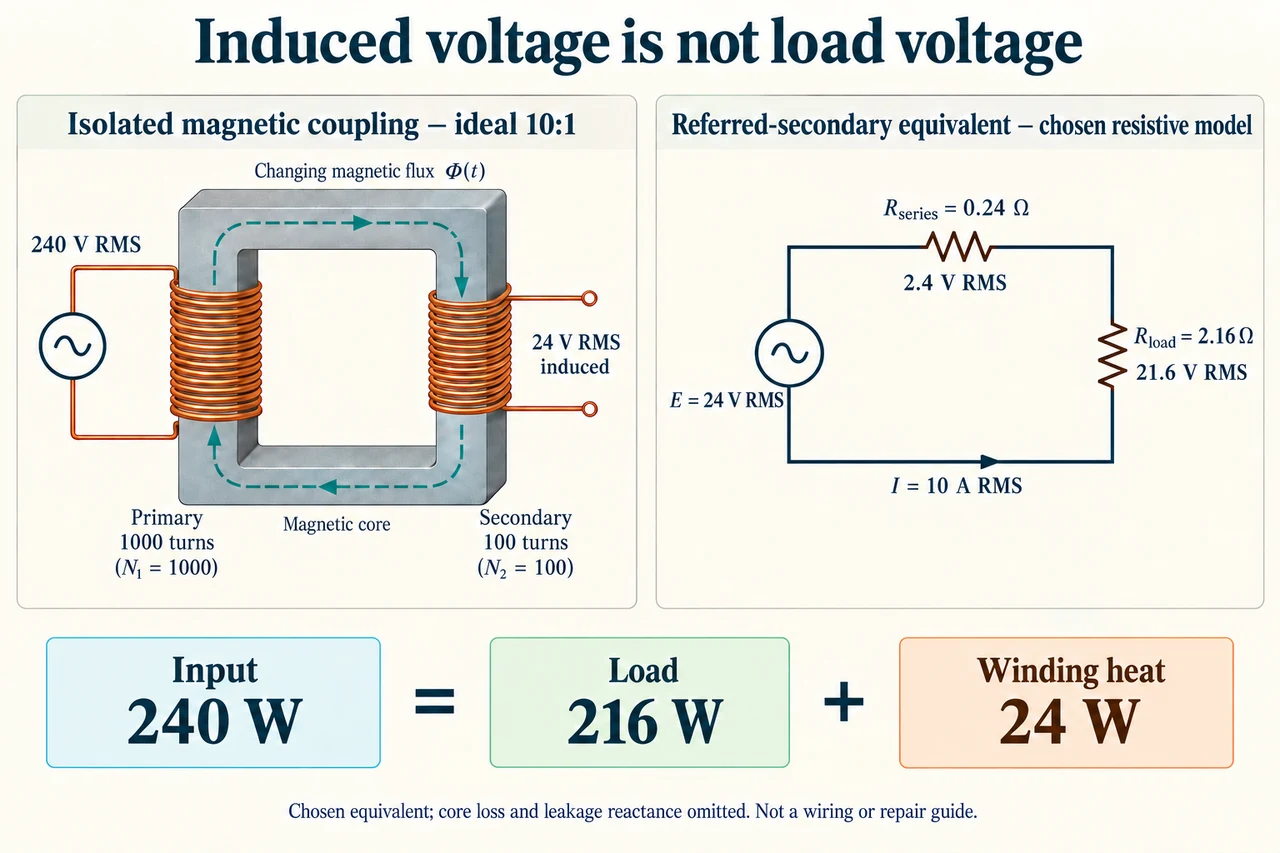
Image: illustration, not a documentary photograph. · Operator-authored generated illustration; scientific model reviewed separately.

Transformers under load: an induced voltage is not the terminal voltage

A transformer transfers electrical energy through a changing magnetic field while keeping its windings electrically separate in the model shown. The primary voltage drives changing flux through a shared core; that changing flux induces an emf in the secondary. Connecting a secondary load changes the electrical demand reflected to the primary, so the source must supply additional power. Current does not jump through the core from one copper wire to the other. The left panel isolates this coupling principle; the right panel is a separate equivalent circuit for calculation, not a wire connecting the two physical windings. Its components represent selected aggregate effects, rather than a buildable equipment layout.

Choose sinusoidal steady operation with 240 V RMS applied to an ideal transformer having 1,000 primary turns and 100 secondary turns. The ideal induced secondary emf is E = 240 × 100/1,000 = 24 V RMS. Add an aggregate winding resistance of 0.24 ohm referred to the secondary and a purely resistive load of 2.16 ohm. Referring resistance means representing both windings' resistive effects on one side of an ideal ratio; it does not mean moving a physical primary wire across the isolation boundary. Neglect leakage reactance, magnetizing current and core losses for this first surrogate. Actual transformers require those effects, waveform information and temperature-dependent properties to predict their behaviour.

The load and aggregate winding resistance are in series in the right-hand equivalent, so current is I = E/(Rseries + Rload) = 24/(0.24 + 2.16) = 10 A RMS. The load terminal voltage is 10 × 2.16 = 21.6 V RMS, while the series winding drop is 10 × 0.24 = 2.4 V RMS. Their sum is the induced 24 V. The turns ratio determines the ideal induced voltage, not a guaranteed loaded terminal voltage after losses. RMS values work in these resistive heating calculations because averaging the square of a sinusoidal current gives the square of its RMS value. Averaging the alternating current itself would give zero and incorrectly predict no heating.

The load receives I²Rload = 10² × 2.16 = 216 W; winding dissipation is I²Rseries = 10² × 0.24 = 24 W. The input to the ideal transformer plus aggregate resistance is E I = 24 × 10 = 240 W, closing the account: 240 = 216 + 24. Primary current in this model is 10 × 100/1,000 = 1 A, so its 240 V source supplies the same 240 W. The complete secondary resistance 2.4 ohm is reflected to the primary as 2.4 × 10² = 240 ohm, also giving 240/240 = 1 A. Model efficiency is useful load power divided by input power, 216/240 = 90%. The 24 W is energy transferred to heating, not energy disappearing.

Now change only the load resistance to 4.56 ohm. Total resistance becomes 4.8 ohm, current falls to 5 A, load voltage is 22.8 V and the winding drop is 1.2 V. Useful power is 5² × 4.56 = 114 W; winding heat is 5² × 0.24 = 6 W; input is 24 × 5 = 120 W. Efficiency rises to 114/120 = 95%, yet the useful output falls from 216 to 114 W. This comparison changes the demanded service. It cannot establish that the second state is better for someone who still requires the original useful output. Lower current reduces resistive losses quadratically, but an efficiency percentage does not specify how much service is delivered.

For a separate sensitivity exercise, keep the original 2.16 ohm load and increase the chosen aggregate winding resistance by 20%, from 0.24 to 0.288 ohm. The new current is 24/2.448 = 9.80392157 A, terminal voltage is 21.17647059 V and useful power is 207.61245675 W. Winding heat becomes 27.68166090 W and input 235.29411765 W, which still equals useful power plus heat. Efficiency is about 88.24%. Increased resistance lowers current at fixed source voltage, so assuming the original 10 A while changing only resistance would describe a different source/load condition. This fixed-resistance surrogate is not a coupled temperature simulation: it cannot forecast thermal runaway, insulation life or a permissible operating temperature.

The scalar sums above rely on a sinusoidal, purely resistive equivalent. With phase-shifted sinusoidal current, average real power is Vrms Irms cos(phi), whereas apparent power is Vrms Irms in VA. Ideal reactive elements exchange energy over a cycle without dissipating that entire VA product as heat. Leakage reactance and excitation branches therefore need phase-aware equations, not a guessed extra resistance or a subtraction of reactive VA from real watts. For distorted waveforms, true power factor is real power divided by apparent power and need not equal one displacement-angle cosine. The plate deliberately omits these branches; its precision comes from declaring those limits, not from claiming all loads behave like resistors. The single current arrow in the equivalent sets a positive reference direction; it does not depict a permanent direct-current flow. Instantaneous current reverses during the alternating cycle, while its RMS magnitude remains the scalar used in the stated resistive heating account.

I would use this model to ask better questions, rather than to prescribe an equipment repair. A reported voltage drop needs evidence about load, waveform, measurement uncertainty, temperature and the condition of connections and insulation, evaluated by qualified people. A measured secondary voltage alone cannot distinguish every cause or confirm isolation safety. Changing equipment solely to improve an efficiency percentage could sacrifice useful service or impose unnecessary material and financial costs. A sound comparison specifies service first, tests the relevant model and considers who bears outages, maintenance costs and access barriers. The two panels show magnetic coupling and a chosen equivalent at different levels of abstraction; neither is an energized test procedure. Image: illustration, not a documentary photograph.

Worked example: For the declared 240 V to 24 V ideal transformer with aggregate referred-secondary resistance 0.24 ohm and resistive load 2.16 ohm, find RMS currents, terminal voltage, useful power, winding dissipation and reflected input resistance. Then change only the load to 4.56 ohm and evaluate the efficiency comparison.

Original series total=2.4 ohm; secondary current=24/2.4 = 10 A RMS. Load voltage=10 × 2.16 = 21.6 V RMS; winding drop=2.4 V RMS.

Useful 216 W and winding 24 W sum to input 240 W. Ideal primary current=10/10 = 1 A. Reflected complete resistance=2.4 × 10²=240 ohm; efficiency 216/240 = 90%.

Changed series total=4.8 ohm; secondary current 5 A, terminal 22.8 V and drop 1.2 V. Useful 114 W plus heat 6 W=input 120 W; primary 0.5 A; efficiency 95%.

The higher efficiency accompanies lower useful service, so it is not an equal-service proof of improvement. Both accounts conserve energy; turns ratio specifies the ideal induced 24 V, not the loaded terminal voltage.

Answer: Original:10 A secondary,1 A primary,21.6 V load,216 W useful and 24 W winding loss. Changed load:5 A secondary,0.5 A primary,22.8 V load,114 W useful and 6 W winding loss. The source/aggregate-loss/load boundary and resistive RMS assumptions are essential.

Check your understanding: Keep the original source and 2.16 ohm load, but increase aggregate resistance 20% to 0.288 ohm. Recompute the account and explain why the original 10 A or a reactive-load VA product cannot simply be reused.

Answer: Total resistance 2.448 ohm gives current 9.80392157 A RMS. Load voltage 21.17647059 V, useful 207.61245675 W and winding 27.68166090 W sum to input 235.29411765 W. Primary current 0.98039216 A; efficiency≈88.2353%. Keeping 10 A would require a different source/load condition because KVL no longer closes at 24 V. The model omits temperature feedback, core loss and leakage reactance. For phase-shifted sinusoidal loads, real average power requires VrmsIrmscos(phi), not the entire VA product; distorted-waveform power factor needs its own definition. These calculations do not provide a temperature limit or repair instruction.

Why: Change only declared terms, re-solve current and close real-energy accounting; distinguish an equivalent and its assumptions from actual equipment diagnosis.