Transformer choices: why a lower full-load loss can cost more energy

By How things work · myAudience

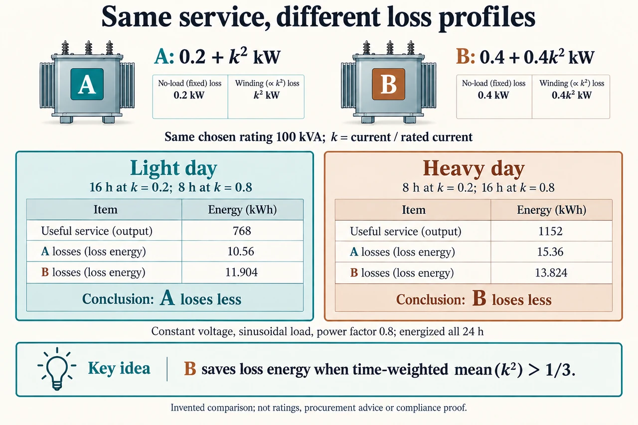
Image: illustration, not a documentary photograph. · Operator-authored generated illustration; scientific model reviewed separately.

Transformer choices: why a lower full-load loss can cost more energy

Choosing a transformer for an electricity service involves more than comparing a full-load efficiency number. Energy losses depend on how long it stays energized and how its current varies. No-load losses occur while the core is excited even when the secondary delivers little useful power; load losses depend strongly on winding current. DOE distinguishes these categories and describes their approximate constant and quadratic behaviour. That description motivates the invented model here, not a universal performance guarantee. Both abstract units on the plate have the same chosen 100 kVA capacity and provide identical service in each comparison. Their drawings do not imply that real products of different construction have equal size, cost or reliability.

Let k be secondary RMS current divided by its chosen rated current. Under constant terminal voltage, it also equals apparent load divided by the common 100 kVA rating. Set A's no-load loss to 0.2 kW and its full-current load loss to 1 kW; choose 0.4 kW and 0.4 kW respectively for B. Their total loss powers are PA = 0.2 + k² and PB = 0.4 + 0.4 k² kW. These constants assume fixed voltage, frequency and temperature, with other losses included or neglected consistently. At k = 1, A loses 1.2 kW and B 0.8 kW, so B appears better at full load. No-load loss nevertheless continues through every energized hour in this model.

The chosen light day has 16 hours at k = 0.2 and 8 hours at k = 0.8. Use sinusoidal loads with fixed power factor 0.8, giving real useful powers of 100 × k × 0.8, or 16 and 64 kW. Both units supply 16 × 16 + 8 × 64 = 768 kWh. A loses 16 × (0.2 + 0.04) + 8 × (0.2 + 0.64) = 10.56 kWh. B loses 16 × (0.4 + 0.4 × 0.04) + 8 × (0.4 + 0.4 × 0.64) = 11.904 kWh. Inputs are consequently 778.56 and 779.904 kWh. A uses less input energy for equal useful service, even though B had lower full-current losses.

Reverse the durations for a heavy day: 8 hours at k = 0.2 and 16 hours at k = 0.8. Useful energy is now 8 × 16 + 16 × 64 = 1,152 kWh for either unit. A loses 8 × 0.24 + 16 × 0.84 = 15.36 kWh; B loses 8 × 0.416 + 16 × 0.656 = 13.824 kWh. Their inputs are 1,167.36 and 1,165.824 kWh, so B avoids 1.536 kWh of losses that day. This is a different but explicitly equal-service comparison between the units. The two days are selected scenarios, not an estimated probability distribution of actual demand, and a site's history could contain many other levels, outages and periods without excitation.

Subtracting the two loss models gives PA − PB = −0.2 + 0.6 k² kW. Over a common energized duration H, B saves loss energy when the time-weighted mean of k² exceeds 1/3. Using the square of mean k would be wrong. For example, constant k = 0.5 over 24 hours has mean square 0.25: A loses 10.8 kWh and B 12.0 kWh. Equal 12-hour blocks at k = 0.2 and 0.8 also have mean k = 0.5 and the same 960 kWh useful service, but mean square is (0.04 + 0.64)/2 = 0.34. A then loses 12.96 kWh and B 12.864 kWh. Variation reverses the preference; peaks affect heating even when daily service and average current match. Algebraically, mean(k²) equals mean(k)² plus variance(k). In the alternating example the deviations from 0.5 are −0.3 and +0.3, so variance is 0.09 and mean square is 0.25 + 0.09 = 0.34. That extra variation term explains why equal averages can hide different integrated heating.

A power-factor transfer exposes another boundary. To supply a fixed 64 kW at power factor 0.8 requires 80 kVA, hence k = 0.8 in this constant-voltage model. At power factor 0.64 the same real power requires 100 kVA, hence k = 1. Current rises by 1/0.8 = 1.25 and the load-loss term grows by 1.25² = 1.5625. A's total loss rises from 0.84 to 1.2 kW and B's from 0.656 to 0.8 kW. Useful real power did not increase. Treating apparent kVA as delivered kW would conceal that distinction. These sinusoidal algebraic cases do not authorize operation at a named rating or prescribe power-factor equipment; waveform, thermal and protection limits require separate professional evidence.

For a deliberately chosen financial scenario, repeat the heavy day on 365 days per year. Avoided loss energy is 1.536 × 365 = 560.64 kWh annually. At a constant chosen price of $0.15/kWh, B saves $84.096 per year relative to A. If B costs an additional $900, simple payback is 900/84.096 = 10.702 years. Over a chosen 20-year horizon with a 3% annual discount rate and end-of-year savings, present value is 84.096 × [1 − 1.03⁻²⁰]/0.03 = $1,251.136; subtracting $900 gives net present value $351.136. Those results omit demand charges, tax, financing, outages, maintenance differences and replacement timing. Repeating the light day instead makes B consume more energy, so a positive simple energy-savings payback no longer exists.

Energy and carbon inventories also need separate boundaries. Choose an additional 1,500 kWh of embodied production energy for B as a sensitivity term, not a measured material footprint. Twenty years of the repeated heavy profile avoids 11,212.8 kWh of operational loss energy, leaving a chosen energy difference of 9,712.8 kWh after that term. Different production and electricity mixes mean this is not a greenhouse-gas calculation. Replacing a functioning installed unit also differs from selecting between two new purchases: premature replacement introduces another counterfactual and disposal cost. I would compare verified load histories, maintainability, material supply, reliability and affordability before selecting. Communities deserve transparent assumptions and a voice in who pays or benefits; no chosen saving alone certifies a responsible purchase. Image: illustration, not a documentary photograph.

Worked example: Calculate both units' losses and input energies for the light and heavy days. Derive the mean-square crossover, then compare constantk 0.5 with equal-durationk 0.2/0.8 at the same daily useful service.

Light: useful 768 kWh; A=16×.24 + 8×.84 = 10.56 kWh and B=16×.416 + 8×.656 = 11.904. Input 778.56/779.904 kWh; A preferred by 1.344 kWh.

Heavy: useful 1152 kWh; A=8×.24 + 16×.84 = 15.36, B=8×.416 + 16×.656 = 13.824. Input 1167.36/1165.824; B preferred by 1.536 kWh.

Difference per hour is−.2+.6 k²; integrate overH hours. B saves when mean(k²)>1/3, assuming identical useful service, excitation duration and chosen loss constants.

Constantk.5 gives mean-square.25 and losses 10.8/12.0. Alternating.2/.8 for 12 hours each gives mean-square.34 and losses 12.96/12.864; both deliver 960 kWh atPF.8. Equal average current does not imply equal losses.

Answer: Neither unit is universally preferable. A wins the light scenario, B the heavy; variance can reverse preference even at equal mean current and useful daily energy. Loss powers must be integrated over duration, not treated as energies or estimated from mean current squared.

Check your understanding: Evaluate selecting B using the chosen heavy-profile financial and embodied-energy scenarios, then challenge the conclusion using the light profile and fixed 64 kW at a power-factor change 0.8→0.64.

Answer: Heavy:560.64 kWh annual savings×$0.15=$84.096/year. Additional$900 gives 10.702-year simple payback. With 20 years/end-of-year savings/3% discount, PV=$1251.136 and netPV=$351.136. Chosen 20-year operational energy savings 11212.8 kWh minus extra embodied 1500 = 9712.8 kWh, not a carbon footprint. Repeated light profile instead increases B losses by 1.344 kWh/day, so the positive energy payback claim fails. At fixed 64 kW, apparent load 80→100 kVA and currentfraction.8→1 make the current-dependent loss 1.5625 times larger; A total.84→1.2 kW and B.656→.8. I would require real profiles, waveforms, prices, material/lifetime evidence and service constraints before a purchase or replacement judgment. The chosen models do not establish compliance or a guaranteed return.

Why: Evaluate an equal-service counterfactual, time-weighted losses, economic and lifecycle boundaries and uncertainty before selecting; invented constants are not actual product measurements.