Three phases, two boundaries: accounting for useful power and line loss

By How things work · myAudience

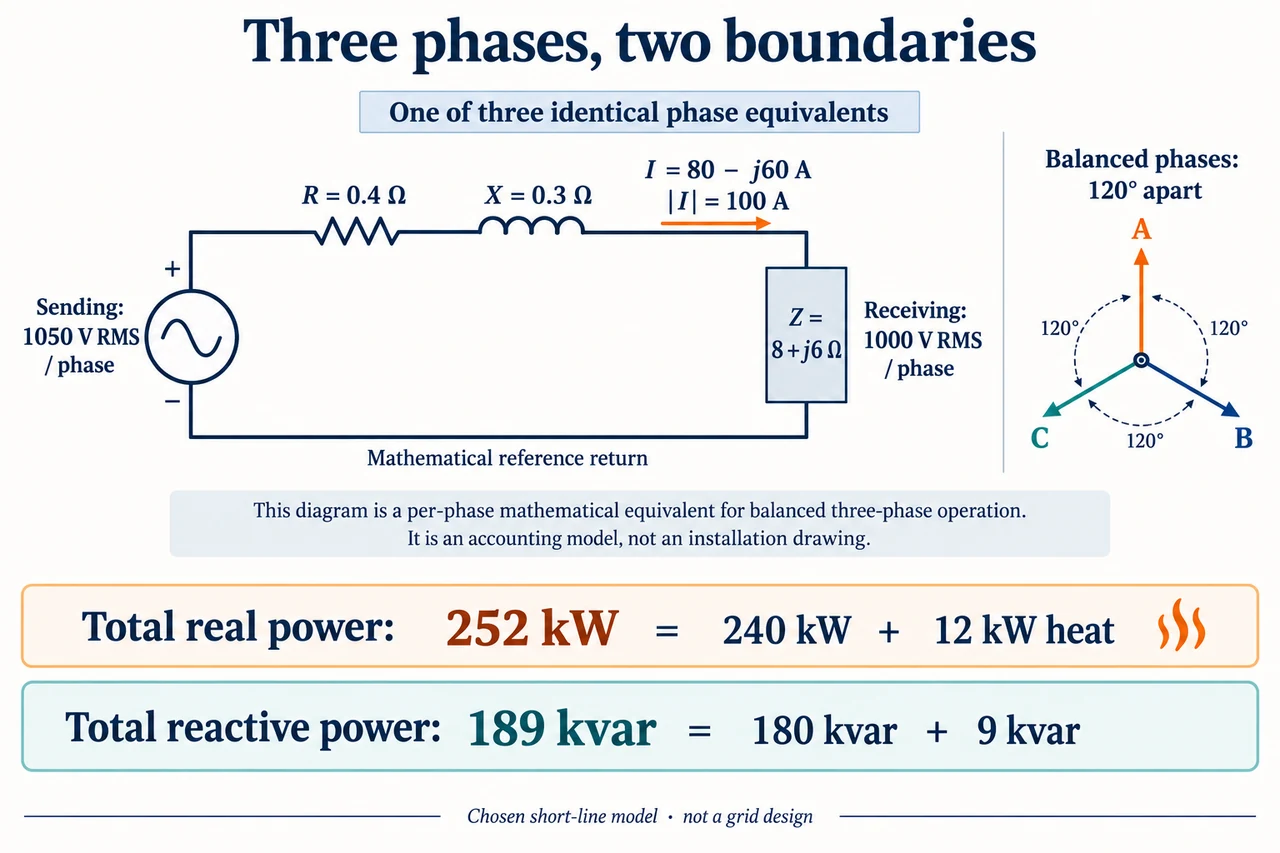
Image: illustration, not a documentary photograph. · Operator-authored generated illustration; scientific model reviewed separately.

Three phases, two boundaries: accounting for useful power and line loss

Transmission serves a useful receiving load; it also transfers energy into heating along the route. To explain both, we must put the accounting boundary in the right place. The earlier transmission lesson used a closed DC equivalent with total loop resistance. Here choose a balanced, sinusoidal three-phase short-line equivalent. Its resistance and reactance are per phase, not the resistance of a two-wire DC loop. Each phase has the same load impedance and equal RMS voltage magnitude, separated by 120 electrical degrees. Treat the receiver as a balanced wye load and use one receiving phase voltage as our zero-angle reference. These choices permit a compact mathematical equivalent; they do not establish an actual installation or include every phenomenon in a real network.

Line-to-line voltage is the difference between two phase-voltage phasors, not the sum of their magnitudes. With phase voltages V at angles 0 and −120 degrees, the squared magnitude of their difference is V² + V² − 2V²cos(120°) = 3V². Thus the line voltage is √3 V, while line current equals the phase current in a balanced wye load. Total real receiving power is three times phase real power: P = 3 V I cos(phi). Total apparent power is 3 V I, and reactive power is 3 V I sin(phi) for this sinusoidal model. The angle phi is between that boundary's voltage and current. At the sending boundary it need not equal the receiving angle. Multiplying a line-to-line voltage by three phase currents without the correct square-root factor would overcount power.

Choose receiving voltage 1,000 V RMS per phase, total useful real power 240 kW, and receiving power factor 0.8 lagging. Current magnitude is 240,000/(3 × 1,000 × 0.8) = 100 A RMS. Because cos(phi) = 0.8 and sin(phi) = 0.6, the phase current is 80 − j60 A relative to the receiving voltage; j denotes a 90-degree rotation in the complex plane, not a physical extra current wire. The chosen receiving impedance is 1,000/(80 − j60) = 8 + j6 ohm per phase. Add line impedance 0.4 + j0.3 ohm per phase. Multiplication gives the line drop (0.4 + j0.3)(80 − j60) = 50 + j0 V. The sending phase voltage is therefore 1,050 V RMS. The plate's closed lower line is a mathematical reference return for one phase equivalent, not a proposed physical neutral conductor.

Complex power at a boundary is three times its phase voltage multiplied by the conjugate of the phase current. Conjugation reverses the current's imaginary sign, so the receiving account is 240 + j180 kVA. At the source it is 3 × 1,050 × (80 + j60) = 252 + j189 kVA. The difference, 12 + j9 kVA, is consistent with 3I²R = 12 kW of resistive heating and 3I²X = 9 kvar of inductive reactive demand. Useful power plus heat closes the real-energy account: 252 = 240 + 12 kW. The reactive account separately closes: 189 = 180 + 9 kvar. A var is not a watt dissipated as heat; ideal reactive elements repeatedly store and return energy. The plate separates these two rows to prevent subtracting reactive power from the useful real output.

For a voltage-transfer comparison, double receiving phase voltage to 2,000 V while holding useful real power, receiving power factor and the line impedance fixed. The current becomes 40 − j30 A, with magnitude 50 A. The line drop is 25 V, sending phase voltage is 2,025 V, and total heat is 3 × 50² × 0.4 = 3 kW. Input real power becomes 243 kW. Line reactive demand is 2.25 kvar, giving total sending reactive power 182.25 kvar. However, the receiving load impedance has become 32 + j24 ohm. This is a changed terminal demand model: it is not the same physical resistor suddenly consuming the same power at twice its voltage. Higher voltage helps this declared comparison, but losses in conversion equipment and actual constraints have been omitted.

A different transfer holds receiving phase voltage at 1,000 V and useful power at 240 kW but changes receiving power factor to unity. Current is then 80 A in phase with receiving voltage, and the load is 12.5 ohm per phase. The line drop is 32 + j24 V; sending voltage is 1,032 + j24 V, whose magnitude is about 1,032.279 V rather than 1,056 V. The latter would incorrectly add perpendicular components as scalar magnitudes. Heating becomes 7.68 kW, while line reactive demand remains 5.76 kvar. Zero reactive demand at the receiver therefore does not make the line reactance disappear or make sending power factor exactly one. Real power entering is 247.68 kW. Lower heating follows the current reduction; it does not certify the safety or suitability of a particular power-factor intervention.

Every numerical result above depends on a balanced sinusoidal steady state with a selected short-line series impedance. A long transmission line may require distributed resistance, inductance and capacitance; shunt charging cannot simply be squeezed into a guessed series resistor. Frequency, temperature, unequal phases and harmonics alter the relationship between current, voltage and losses. Network stability, insulation, mechanical clearance, protection and outage contingencies can impose constraints even when this heat account looks attractive. The current arrow defines a positive phasor reference; instantaneous AC reverses during a cycle. The little three-phase inset explains relative angles, while the equivalent supplies a calculation boundary. Neither depicts a complete field wiring or a construction plan.

An evidenced decision must compare the service delivered and the people affected, not just pick the smallest heat figure. The doubled-voltage case retains 240 kW at the receiver but assumes a different load interface; a real comparison would include conversion losses, cost, materials, inspection, reliability and environmental consequences along the route. Existing corridors may reduce some new land disturbance while raising other clearance or community concerns. Communities paying for infrastructure may differ from those receiving its benefit. We should request route-specific evidence and assess alternatives such as demand reduction and reinforcement before inferring that a lower model loss is the best public choice. The image's separate real and reactive ledgers are tools for scrutinizing that evidence, not a substitute for it. Image: illustration, not a documentary photograph.

Worked example: For the declared balanced short-line model, calculate receiving and sending real and reactive powers. Evaluate the doubled-voltage and unity receiving power-factor transfers, explaining what changes at the load.

At receiving 1,000 V per phase and power factor 0.8, useful total power 240 kW requires current magnitude 100 A. Its phasor is 80 − j60 A. Load impedance is 8 + j6 ohm; multiplying line impedance 0.4 + j0.3 ohm by current gives 50 V in-phase drop and sending voltage 1,050 V per phase. Receiving line-to-line voltage is 1,732.051 V.

Receiving complex power is 240 + j180 kVA; sending complex power is 252 + j189 kVA. Their difference separates 12 kW heat from 9 kvar reactive demand. Independently check 3 × 100² × 0.4 = 12,000 W and 3 × 100² × 0.3 = 9,000 var. Sending apparent power 315 kVA is neither useful real power nor dissipated heating.

Doubling receiving phase voltage at fixed useful power and receiving power factor gives current 40 − j30 A, load 32 + j24 ohm, drop 25 V and sending voltage 2,025 V per phase. Heat is 3 kW and line reactive demand 2.25 kvar; sending complex power is 243 + j182.25 kVA. The changed load impedance is essential: a fixed load impedance would not preserve the useful service.

For unity receiving power factor at the original voltage and useful power, current is 80 A and load 12.5 ohm. The drop is 32 + j24 V, making sending voltage 1,032 + j24 V with magnitude 1,032.279 V per phase. Input complex power is 247.68 + j5.76 kVA. Line reactive demand remains despite zero receiver reactive demand. The source and receiver power factors differ.

Answer: The accounts close separately at each boundary. Real input equals useful output plus heat; reactive demand must not be called additional heat. The altered terminal conditions explicitly change the load in each transfer. This model supports those calculations, while protection, distributed-line behaviour, conversion losses and route or community evidence remain outside it.

Check your understanding: A learner adds 1,032 + 24 to find sending RMS voltage and calls the line’s 5.76 kvar a 5.76 kW heat loss in the unity receiving power-factor case. Correct both errors and give a bounded conclusion.

Answer: The two voltage components are perpendicular phasor components, so magnitude is √(1,032² + 24²) = 1,032.279 V per phase. Line heating is 7.68 kW; reactive demand is 5.76 kvar. They are different quantities. At the declared fixed useful receiving power and voltage with the changed load, lower current lowers resistive heating. It does not establish a suitable real network design. Unity receiver power factor does not force unity sending power factor.

Why: A valid evaluation keeps phasor geometry, real energy and reactive exchange separate. Stating what is held fixed exposes the altered load assumption and prevents an efficiency calculation from becoming an unsupported grid-design claim.