Which yield improvement actually reduces resource use?

By How things work · myAudience

myAudience original rendered teaching illustration. Image: illustration, not a documentary photograph. · myAudience educational illustration; no certification or manufacturing qualification is implied.

Which yield improvement actually reduces resource use?

A chip lot can pass through several filters: surviving fabrication defects, meeting packaging requirements and meeting final electrical criteria. A percentage means little without naming the entering population and the criteria. More passing dies are useful only when they provide the required function. In this lesson we hold that intended function constant by explicit assumption while comparing three fictional design/process scenarios. Critical area is the area vulnerable to the chosen defect mechanism; it need not equal the whole geometric die area. We do not derive the number of candidate dies from wafer diameter or assume that shrinking critical area automatically creates more wafer positions.

For a simplified Poisson model, the mean count of killing defects is λ = A_c D, with critical area A_c in cm² and defect density D in cm⁻². The units cancel. The probability of zero such events is exp(−λ). This gives one defect-survival factor, not every form of manufacturing success. The model assumes a constant density and spatially uncorrelated pointlike defects that cause failure within the relevant critical area. Clusters, systematic geometry errors, redundant circuits and non-killing defects can invalidate that description. The historical MIT teaching model is a way to reason from declared assumptions, not a contemporary factory-yield estimate.

Choose 500 candidate dies and A_c = 0.8 cm² with D = 0.3 cm⁻². The mean is 0.24, so defect survival is approximately 0.786628. The expected number entering packaging is 393.314. Give packaging a conditional pass fraction of 0.95 among those entering it, and final test a conditional pass fraction of 0.98 among packaged passes. Expected qualified output is 500 × exp(−0.24) × 0.95 × 0.98, or 366.175. Multiplying these explicitly conditional factors is the probability chain; it does not assert that all defects and all packaging failures are physically independent.

The fractional output is a planning average across repeated comparable lots, not a fraction of a physical die on one wafer. A realised lot contains whole objects and fluctuates. Also, a passing final test does not promise unlimited service life or detect every possible fault. Different tests may screen different characteristics, and a packaging change can alter both pass criteria and failure mechanisms. An expected-count calculation should therefore accompany test definitions, calibration evidence and a clear separation between prediction and observation. Replacing the word expected with guaranteed would be a substantive error even if every arithmetic step stayed unchanged.

Now declare a narrow energy boundary: 200 kWh of fixed preparation/fabrication energy, 0.05 kWh per initial candidate for a chosen earlier screening stage, and 0.10 kWh for each expected die entering downstream packaging. The baseline total is 200 + 25 + 39.331 = 264.331 kWh. Dividing that expected total by 366.175 expected qualified dies gives 0.721871 kWh per expected qualified die. This is a ratio of planning totals, not the statistical expectation of a random per-lot ratio. Water, gases, upstream materials, device use and end-of-life are excluded; the result cannot be called a complete environmental footprint.

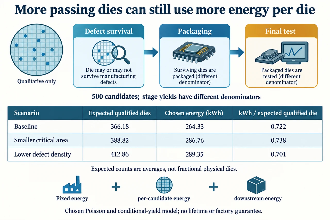
Alternative A reduces critical area to 0.6 cm² at the same density, with a chosen additional fixed energy cost of 20 kWh. The expected qualified output rises to 388.818, but total energy becomes 286.764 kWh and intensity rises to 0.737526. Alternative B retains 0.8 cm² but halves defect density to 0.15 cm⁻², also costing 20 extra fixed kWh. Its output is 412.861 and energy 289.346 kWh, giving 0.700831. Under this boundary B improves intensity, while A worsens it despite producing more qualified dies. Neither extra-energy number is a measured cost of industrial shrinking or cleaner processing.

The plate shows the three conditional stages and a table of rounded expected outputs, energy totals and ratios. Its wafer icon is qualitative: dots do not represent a counted production map. The table’s 0.722, 0.738 and 0.701 are rounded from the unrounded calculations in the text. Arrows show population flow, not automatic repair. The fictional energy account includes consumption on dies that later fail; discarding their material does not undo already spent energy. The design comparison would need to be recalculated if a changed function, lifetime or useful-work denominator made equal die counts an unfair comparison.

A responsible recommendation retains these boundaries and seeks evidence beyond a yield headline. EPA’s current page describes process emissions that vary with gases, tools, process choices and abatement; our electrical-energy model does not estimate those emissions. Procurement can also weigh access, workforce conditions, resource demand and supportable device lifetime. An unfamiliar shared wafer-loss factor reduces useful output while fixed upstream energy remains spent, illustrating why a good local yield does not establish good system performance. Prefer B only under the declared equal-function and resource assumptions; revise that preference when independently measured evidence changes the comparison. Image: illustration, not a documentary photograph.

Worked example: Compare the three chosen scenarios using 500 candidates, conditional packaging yield 0.95, conditional final-test yield 0.98, fixed baseline energy 200 kWh, 0.05 kWh per initial candidate and 0.10 kWh per die surviving the chosen defect mechanism. Baseline uses critical area 0.8 cm² and density 0.3 cm⁻². A uses 0.6 cm² at the same density; B uses 0.8 cm² at density 0.15 cm⁻². Both alternatives add 20 fixed kWh. Assume the intended delivered function is held constant.

For each scenario compute λ = A_c D and Y = exp(−λ). The dimensionless means are 0.24, 0.18 and 0.12; the survival probabilities are 0.7866278611, 0.8352702114 and 0.8869204367. These are chosen-model probabilities, not measured percentages. They describe zero killing defects under the Poisson assumptions; other yield losses are deliberately handled by separately stated conditional factors.

Expected downstream entrants are 500Y: 393.3139305, 417.6351057 and 443.4602184. Expected qualified output multiplies each by 0.95 × 0.98 = 0.931, giving 366.1752693, 388.8182834 and 412.8614633. The packaging denominator is surviving dies, and the final-test denominator is packaged passes. Their product is appropriate because those conditional populations are explicitly defined; blindly multiplying headline percentages with unrelated denominators would not be justified.

Count energy on the stages where it is incurred. Initial screening contributes 500 × 0.05 = 25 kWh in every case. Downstream energy is 0.10 times the expected entrants, not qualified output: some entrants consume energy and later fail. Add fixed energy of 200, 220 and 220 kWh. Totals are 264.3313931, 286.7635106 and 289.3460218 kWh. Dividing by the matching expected qualified totals gives 0.7218712327, 0.7375257872 and 0.7008307812 kWh per expected qualified die.

The evaluated answer is not simply choose the largest yield. A produces more expected qualified dies than baseline but increases this energy intensity by about 2.17%; B lowers intensity by about 2.92%. Under an explicitly unchanged intended function and this resource boundary, B is preferred for energy per qualified output. However, a different lifecycle, test coverage, service reliability or upstream material burden can reverse a broader decision. The model establishes only its own narrow ranking; assessors should reject a claim that it proves the best semiconductor technology or guarantees a real lot’s output.

Answer: Baseline/A/B expected qualified output is 366.175/388.818/412.861; the respective chosen energy intensities are 0.721871/0.737526/0.700831 kWh per expected qualified die. B improves the declared intensity, while A worsens it despite higher output. The conclusion is conditional on equal intended function and the stated resource boundary.

Check your understanding: Introduce a chosen 0.90 wafer-survival factor before the earlier screening and packaging stages, independent of the stated defect model. All 500 initial candidates have already incurred fixed energy, but only surviving wafers’ candidates incur the 0.05 kWh screening term and enter the downstream stages. Recalculate baseline and B expected qualified output, energy and intensity. Does B remain preferable within this boundary?

Answer: Baseline output is 0.90 × 366.1752693 = 329.5577424; B output is 0.90 × 412.8614633 = 371.5753170. Screening now costs 450 × 0.05 = 22.5 kWh. Baseline downstream energy is 0.10 × 0.90 × 393.3139305 = 35.3982537 kWh; B downstream energy is 39.9114197 kWh. Fixed energy remains 200 or 220, so totals are 257.8982537 and 282.4114197 kWh. Intensities are approximately 0.782559 and 0.760038 kWh per expected qualified die. B still has the lower declared intensity, but both are worse than their no-wafer-loss counterparts. Multiplying the entire energy total by 0.90 would incorrectly erase energy already spent upstream. This chosen shared factor is not an estimate of a real factory’s wafer survival.

Why: Separate fixed sunk energy from downstream population-dependent terms; use matching expected denominators and keep the new loss factor’s position explicit.