AI matrix work: reuse, arithmetic intensity and bounded throughput

By How things work · myAudience

Original myAudience educational illustration. Image: illustration, not a documentary photograph. · myAudience educational illustration; no vendor affiliation or measured hardware performance is implied.

AI matrix work: reuse, arithmetic intensity and bounded throughput

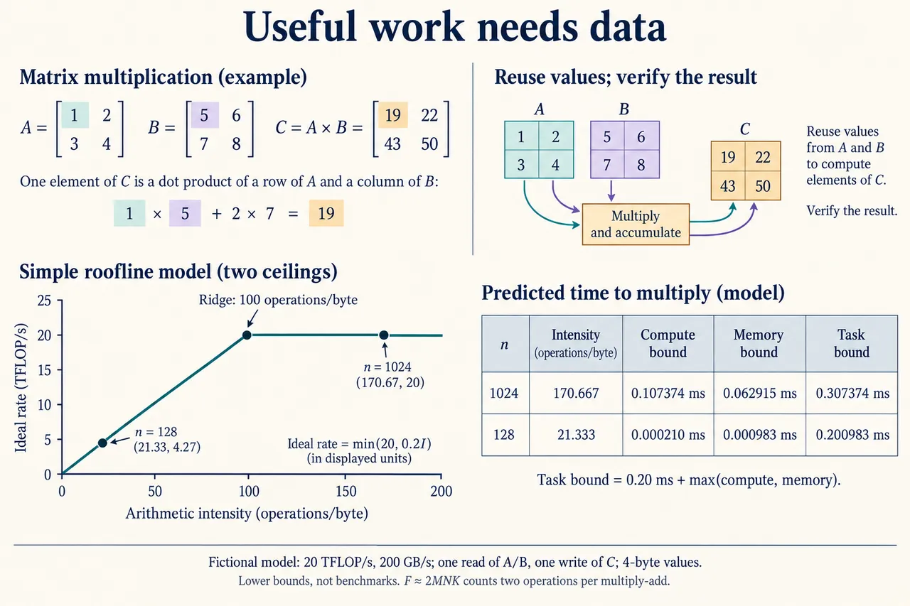
Dense matrix multiplication is an important building block in many machine-learning systems, although an AI application also contains control, indexing, communication and operations that are not matrix products. For C = AB, each output combines a row of A with a column of B. Our original example uses A with rows [1, 2] and [3, 4], and B with rows [5, 6] and [7, 8]. The top-left result is 1 times 5 plus 2 times 7, or 19; the full output is [[19, 22], [43, 50]]. This small calculation establishes what values mean before discussing faster hardware. An accelerator's impressive advertised operation rate is irrelevant if the implemented indexing or accumulation computes a different result.

Performance accounting requires a declared operation convention. If A is M by K and B is K by N, the usual high-level convention counts K multiply-accumulates per output and two operations per multiply-add, giving F = 2MNK. That is a useful leading-order work convention, not an exact count of every scalar addition, instruction or initialization operation in our small two-by-two example. A direct scalar dot product can use K multiplications and K minus one additions; an accumulator initialized to zero has another description. Floating-point fused operations also differ in rounding from separately rounded multiplication and addition. Check a suitable reference and error tolerance, with like precision and a justified numerical requirement, before interpreting any speed comparison.

A tiled algorithm assigns portions of the output to cooperative groups and repeatedly reuses input values while accumulating those outputs. A row value can contribute to several neighboring results rather than being fetched independently for each result. This is a way of organizing work and data, not proof that a particular implementation achieves the smallest possible DRAM traffic. Registers, shared workspace and caches may support reuse at different levels; tile shapes, remaining edge values and capacity limits matter. Correct cooperation requires each group to know which data are available and which output positions it owns. Increasing reuse at one level can add overhead or exhaust a limited resource elsewhere, so the design remains something to validate and measure.

For a simple lower-bound account, stipulate four-byte elements, C = AB with no previous C to read, one read of every A and B element at our chosen memory boundary and one write of every output. Then Q = 4(MK + KN + MN) bytes. This deliberately favorable account excludes repeated loads, initialization, temporary arrays, cache-line inefficiency and protocol traffic. Arithmetic intensity I = F divided by Q is measured in operations per byte at that boundary. Changing the boundary or precision changes its meaning. A larger memory capacity does not alter this ratio automatically; a layout or algorithm must actually exploit the available space to reduce observed movement.

Suppose a fictional device sustains at most P operations per second for the same declared arithmetic type and at most B bytes per second at the chosen boundary. The ideal useful rate cannot exceed the smaller of P and B times I. Equivalently, its kernel time is bounded below by the larger of F divided by P and Q divided by B. The crossing intensity P divided by B is the ridge of this simplified two-ceiling model. It diagnoses a possible limiting resource, not an achieved speed. Dependencies, inadequate parallel work and instruction overhead can push performance below both ceilings. Real overlapping transfers and computation also need evidence; the model's maximum is an optimistic bound, not an instruction to omit elapsed time.

Our invented comparison fixes P at 20 trillion operations per second, B at 200 billion bytes per second and a separate, non-overlappable launch and coordination cost of 0.20 milliseconds. Decimal units are used consistently. A square matrix of side 1024 has F = 2,147,483,648 and Q = 12,582,912 bytes, so I is about 170.667 operations per byte. The compute bound is about 0.107374 milliseconds and the memory bound 0.062915 milliseconds. Adding the fixed term to the larger gives an ideal task lower bound of about 0.307374 milliseconds. A square matrix of side 128 has I about 21.333, so its memory bound exceeds its compute bound, yet the total lower bound is about 0.200983 milliseconds because the fixed term dominates.

Inference serving must connect such kernel accounting to an individual request. Combining requests into a larger batch can expose more reuse and parallel work, but waiting for a batch can delay someone who needs a quick answer. Larger batches also consume memory and may create different scheduling or data-isolation obligations. Training and inference are not interchangeable performance tasks: their computation, retained state and quality checks differ. Neither a throughput gain nor a lower modeled kernel time establishes a shorter response for every user. A fair comparison declares the task, numerical accuracy, batch policy and complete timing boundary. Resource claims additionally require a complete meter boundary; this plate supplies no measured energy or environmental ranking.

Consider the 128 case again. Doubling only the compute ceiling does not change its modeled task lower bound, because the memory term remains larger. Doubling only bandwidth lowers the memory term from 0.00098304 to 0.00049152 milliseconds, giving a total of 0.20049152 milliseconds, nowhere near half the original task time. The fixed 0.20 milliseconds survives both interventions. This counterexample answers why buying more arithmetic capability can disappoint a service whose real limits lie elsewhere. The sensible next step is to measure the actual task and its accuracy before choosing an intervention. Image: illustration, not a documentary photograph. The graph and tiled calculation depict a hypothetical model; they are neither a hardware floorplan nor a benchmark result.

Worked example: Stipulate square, single 4-byte-element GEMM C = AB. Use the leading-order convention of two operations per multiply-add; ignore lower-order work, initialization and other instructions. Read each A/B element once and write C once at a declared memory boundary. Hypothetical matched arithmetic ceiling 20 × 10¹² operations/s and bandwidth 200 × 10⁹ bytes/s, plus 0.00020 s unavoidable launch/coordination. Compare n = 1024 and n = 128.

Fix both the task and arithmetic convention. For a square C = AB of side n, use F = 2n³ as the leading-order two-operations-per-multiply-add convention. This is not an exact count of every instruction or lower-order initialization operation. With four-byte elements and ideal one-time input reads plus one output write, Q = 4(n² + n² + n²) = 12n² bytes. This favorable Q must not be called measured DRAM traffic.

At n = 1024, F = 2,147,483,648 operations and Q = 12,582,912 bytes. Arithmetic intensity F/Q = n/6 = 170.6666667 operations per byte. At n = 128, F = 4,194,304 operations and Q = 196,608 bytes, giving 21.3333333 operations per byte. Both use the same precision, operation convention and traffic boundary; mixing a different tensor arithmetic peak into one comparison would invalidate it.

The fictional ceilings are P = 20 × 10¹² operations/s and B = 200 × 10⁹ bytes/s, using decimal prefixes. Their ratio P/B = 100 operations/byte is the ridge. The ideal useful rate is at most min(P, B × I); equivalently kernel time is at least max(F/P, Q/B). This optimistic lower bound permits perfect overlap of compute and memory work. It supplies no proof that a kernel reaches either advertised ceiling.

For n = 1024, F/P = 0.0001073741824 seconds = 0.1073741824 ms. Q/B = 0.00006291456 seconds = 0.06291456 ms. The compute term is larger. Adding the stipulated, non-overlappable 0.20 ms launch/coordination term gives 0.3073741824 ms. A higher real traffic count, dependencies or other overhead would raise elapsed time, not violate the lower-bound reasoning.

For n = 128, compute time is 0.0002097152 ms and memory time 0.00098304 ms. Memory is the larger kernel term, but neither is the dominant end-to-end contribution: the fixed 0.20 ms term is. Total lower bound is 0.20098304 ms. Saying this small task is memory limited without mentioning the fixed term would be an incomplete explanation of the user-visible task boundary.

Doubling only compute leaves the n = 128 total unchanged because its memory term still exceeds compute. Doubling only bandwidth gives memory time 0.00049152 ms, still above compute, and total 0.20049152 ms. Neither intervention halves the task bound. The reasoned choice therefore begins with measuring the complete task and preserving numerical meaning, then testing an intervention such as reduced setup or justified batching; it does not begin with buying a larger arithmetic peak.

Answer: The declared n = 1024 task has an ideal lower bound of 0.3073741824 ms, while n = 128 has 0.20098304 ms. Compute dominates the large kernel account; memory dominates the small kernel account, but the fixed 0.20 ms term dominates the small complete task. Doubling arithmetic alone cannot improve that small-task bound. Doubling bandwidth changes it only to 0.20049152 ms. All figures are conditional model results, not hardware benchmarks, accuracy guarantees or an energy comparison.

Check your understanding: For n = 128, double the compute ceiling alone, then separately double bandwidth. Does either halve the stipulated end-to-end lower bound? Explain why equal precision, equal task and launch/measurement boundaries matter.

Answer: Doubling compute alone leaves memory time 0.00098304 ms dominant and the total unchanged. Doubling bandwidth alone halves memory time to 0.00049152 ms, still above compute time 0.0002097152 ms, giving total 0.20049152 ms. This is nowhere near half because the fixed 0.20 ms dominates. Comparisons must match task and allowed numerical error and include actual traffic, scheduling and user wait.

Why: A valid comparison retains the declared task, precision and boundary; a theoretical limiting-resource account is not an observed user-time or energy guarantee.