Seasonal service: weight heat, capacity and backup rather than headline COP

By How things work · myAudience

Original myAudience educational illustration. Image: illustration, not a documentary photograph. · myAudience educational illustration; no measured product performance or installation qualification is implied.

Seasonal service: weight heat, capacity and backup rather than headline COP

A seasonal heating question combines many operating conditions and asks about a service delivered over time. An instantaneous heating COP divides heat by electrical input over a declared interval and boundary. A period ratio divides the sum of useful heat by the sum of all included electricity. It is usually not the arithmetic mean of several COP values. A period with high demand or substantial backup input can contribute disproportionately to the denominator. The fictional bin model here teaches that accounting distinction; it is not a regulated SCOP or HSPF rating, a weather record, or a prediction for an actual home.

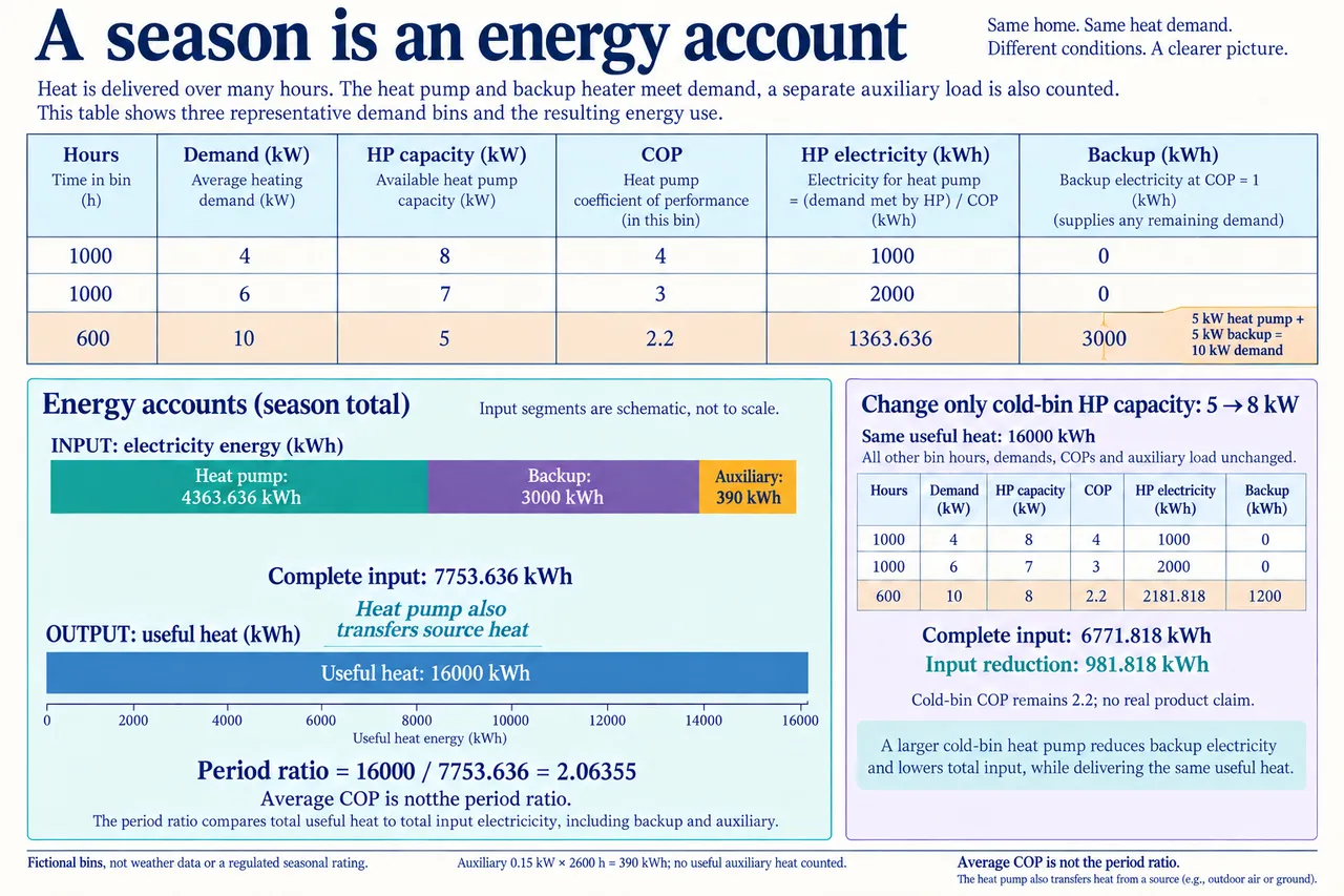
The example stipulates three operating bins rather than importing a real climate. The first lasts 1000 hours with a 4 kW heating demand, heat-pump capacity of 8 kW and COP of four. The second lasts 1000 hours with 6 kW demand, 7 kW capacity and COP of three. The third lasts 600 hours with 10 kW demand, only 5 kW heat-pump capacity and COP of 2.2. Capacity means available heat-output power in that bin, not electric input or stored energy. Each bin is assumed steady. The heat pump can meet up to the smaller of demand and capacity; a stipulated resistance backup with COP one supplies the remaining heat.

For this teaching account, all listed heat reaches the selected useful-delivery boundary, with no distribution loss. The bin COPs exclude a separate 0.15 kW auxiliary electrical load operating throughout all 2600 hours. Its energy is explicitly outside useful delivered heat; it must not be counted again as a hidden benefit. This convention is a stipulated boundary, not a claim about where every real fan motor releases heat. In the first two bins, the pump supplies the whole demand. In the third, it provides 5 kW and backup provides another 5 kW, so the service can be met even though the pump alone lacks sufficient capacity.

Multiply each rate by its bin’s duration before summing. Useful heat is 4000 + 6000 + 6000 = 16000 kWh. Heat-pump electricity is 4000/4 + 6000/3 + 3000/2.2 = 4363.636 kWh. The third bin’s remaining 3000 kWh comes from resistance backup and requires 3000 kWh of electricity in the stipulated model. Auxiliary input is 0.15 × 2600 = 390 kWh. Total input is therefore 7753.636 kWh, giving a useful period ratio of approximately 2.06355. Averaging four, three and 2.2 gives 3.0667, but that number omits both how much heat each period supplies and the backup and auxiliary contributions.

A narrow counterfactual raises only the third-bin heat-pump capacity to 8 kW while keeping its COP at 2.2 and all other data unchanged. The pump now supplies 4800 kWh in that bin and backup supplies 1200 kWh. The complete electricity sum becomes 6771.818 kWh, reducing input by 981.818 kWh for the same 16000 kWh of useful heat. The improvement comes from substituting heat-pump delivery for stipulated COP-one backup, not from inventing a larger COP. This calculation says nothing about whether a particular larger unit keeps the same performance, whether its mild-condition cycling changes, or whether purchase, maintenance and installation costs are justified.

Real operation can contain events that the bins omit. An outdoor exchanger may accumulate frost, and a defrost operation can temporarily change the heat and electrical accounts. Part-load controls, cycling, distribution loss and changing source or delivery conditions also require measurements or a justified model. The cited 2024 laboratory report investigated selected systems and conditions, with explicit limitations on extending results to annual performance, backup energy or distribution losses. Our made-up bins are not disguised data from that study. A credible future analysis would define the complete meter boundary and record enough time-dependent service and input evidence to evaluate those omitted effects.

Energy accounting is one part of a decision, not a complete affordability or environmental verdict. A smaller input sum does not supply an electricity tariff, carbon intensity, equipment lifetime or repair burden. Peak electrical demand may matter differently from total kilowatt-hours, while comfort and accessibility determine whether a service is acceptable. Comparisons should supply those additional data and a matched useful task, rather than assume that one ratio represents every household’s experience. This example deliberately makes no current rebate, product or emissions claim. It encourages a transparent case comparison with declared uncertainties before turning a model into a recommendation.

The worked distribution-loss example moves the useful boundary. If ten percent of the model’s 16000 kWh fails to reach rooms while all electrical inputs remain unchanged, room delivery is 14400 kWh and the new boundary ratio is approximately 1.85719. That is less useful service; it cannot be advertised as a measured change in device COP or as proof of equal comfort. Providing the original room heat would require another explicitly modelled intervention or input. Image: illustration, not a documentary photograph. The table and energy totals are original teaching values, not a weather sample, equipment rating or instructions for refrigerant or electrical work.

Worked example: Use three fictional heating bins: (1000 h, demand 4 kW, capacity 8 kW, COP 4); (1000 h, demand 6 kW, capacity 7 kW, COP 3); (600 h, demand 10 kW, capacity 5 kW, COP 2.2). Backup has COP one; separate non-useful auxiliary input is 0.15 kW throughout. All model heat reaches the useful boundary. Calculate the period service ratio and the counterfactual with third-bin capacity 8 kW only.

Within each bin, heat-pump output power is min(demand, available capacity). The pump therefore supplies 4, 6 and 5 kW, while backup supplies 0, 0 and 5 kW. This rule states how the invented service is met; it does not describe an actual controller or establish that a product can sustain these outputs. Heat output and electrical input are different quantities.

Convert rates to energy using the stated durations. Useful heat is 4 × 1000 + 6 × 1000 + 10 × 600 = 16000 kWh. Heat-pump heat contributions are 4000, 6000 and 3000 kWh. Divide each by its own COP before summing electricity: 1000 + 2000 + 1363.636364 = 4363.636364 kWh. Backup supplies 3000 kWh of heat and uses 3000 kWh electricity.

The auxiliary account is 0.15 × (1000 + 1000 + 600) = 390 kWh, explicitly not useful heat at this chosen boundary. Complete input is 4363.636364 + 3000 + 390 = 7753.636364 kWh. The useful period ratio is 16000/7753.636364 = 2.063547895. Arithmetic mean COP is 3.0667, which ignores heat weighting, backup and auxiliaries and therefore answers a different question.

Change only the third-bin heat-pump capacity to 8 kW. At the unchanged COP of 2.2 it supplies 8 × 600 = 4800 kWh heat and uses 2181.818182 kWh electricity; backup now supplies and consumes 1200 kWh. Other bin and auxiliary accounts stay fixed. Total input is 1000 + 2000 + 2181.818182 + 1200 + 390 = 6771.818182 kWh.

Useful heat remains 16000 kWh, so the comparison holds that service constant. The counterfactual ratio is 2.362733253 and input reduction is 7753.636364 − 6771.818182 = 981.818182 kWh. This improves the model by replacing part of COP-one backup. It is not proof that installing a larger unit preserves COP, cycling, cost or environmental impact; those assumptions must be independently tested.

Finally change the useful-delivery boundary: lose ten percent of gross model heat before rooms while retaining input. Room heat becomes 14400 kWh and ratio 14400/7753.636364 = 1.857193106. Less delivered room heat is not equivalent comfort or a newly measured device COP. Declare omitted defrost, distribution and time-dependent effects and collect matched service and complete-input evidence before recommending a real intervention.

Answer: The fictional service delivers 16000 kWh using 7753.636364 kWh complete electricity, giving a period ratio 2.063547895. Raising only cold-bin capacity to 8 kW with unchanged COP yields the same heat using 6771.818182 kWh, ratio 2.362733253 and input reduction 981.818182 kWh. A ten-percent loss before the room boundary instead gives 14400 kWh useful heat and ratio 1.857193106, with reduced service. None is a regulated seasonal rating, measured product result or equal-comfort guarantee.

Check your understanding: Keep the original three bin durations, demands, heat-pump capacities and 0.15 kW non-useful auxiliary load. Change only the cold-bin COP from 2.2 to 2.5; its heat-output capacity remains 5 kW against 10 kW demand. Calculate complete period electricity and useful-service ratio. Explain why backup heat cannot be removed merely because the COP improved.

Answer: Cold-bin heat-pump output is still 5 × 600 = 3000 kWh; electricity is now 3000/2.5 = 1200 kWh. Backup must still supply the other 5 × 600 = 3000 kWh and uses 3000 kWh at COP one. Complete input is 1000 + 2000 + 1200 + 3000 + 390 = 7590 kWh. Useful heat stays 16000 kWh, giving ratio 16000/7590 ≈ 2.108037. Input falls by 1800/11 ≈ 163.636364 kWh versus the original case. COP relates heat to input; it does not increase the stipulated heat-output capacity. Removing backup would leave half the cold-bin demand unmet.

Why: A new COP changes electrical input for the same heat-pump delivery, while capacity continues to limit cold-bin output. Keep backup and auxiliary accounts, preserve equal useful service and sum energies before dividing rather than averaging COP values.