Solar inverters: clipping is not conversion heat

By How things work · myAudience

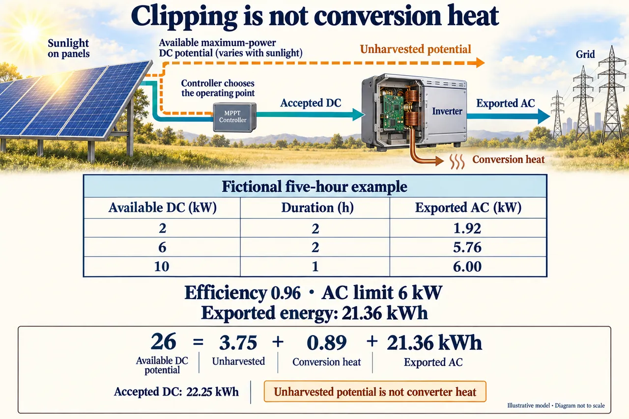
Original myAudience educational illustration. Image: illustration, not a documentary photograph. · myAudience educational illustration; fictional model, no certified rating or installation qualification implied.

Solar inverters: clipping is not conversion heat

A solar array and an inverter have different jobs and different limits. The array converts part of the incoming light into electrical output; its current-voltage characteristic depends on conditions and the chosen operating point. Its largest available DC power at a particular moment is not the same as the power actually drawn. The inverter accepts DC input and produces AC output within its own constraints. A panel nameplate describes specified test conditions, rather than a promise that the array produces that power throughout the day. This lesson follows an original, deliberately simplified time-bin account to separate available maximum-power potential, accepted DC energy and delivered AC energy.

Switching and maximum-power tracking explain different parts of the causal chain. Semiconductor switches regulate an electrical waveform; filtering suppresses unwanted switching components so the converter can provide suitable AC. A maximum-power controller chooses or adjusts the array operating point to seek useful output under changing conditions. These functions can be integrated in different hardware arrangements; the controller in the illustration identifies a function, not a mandatory separate box. A grid-following inverter also needs an external voltage reference for its synchronization. Converting DC to AC therefore does not by itself establish that the same installation can provide approved, stable electricity to isolated loads during a grid outage.

In the teaching model, available DC power is P_available, the constant conversion efficiency is eta, and the allowed AC output is P_cap. For each steady bin, exported active power is min(eta × P_available, P_cap). If the cap binds, we stipulate that the controller reduces the accepted DC power rather than dissipating all unused potential inside the inverter. Accepted power is then exported power divided by eta. This simplified rule excludes voltage windows, current limits, auxiliaries, reactive service and changing efficiency. Real converters can have more restrictive operating envelopes. The equation is an explicit original surrogate for this exercise, not the current PVWatts algorithm or a measured product curve.

Take three available-DC bins of 2, 6 and 10 kW lasting 2, 2 and 1 hours. With eta = 0.96 and a 6 kW AC cap, conversion without the cap would give 1.92, 5.76 and 9.6 kW. Applying the cap within each bin gives 1.92, 5.76 and 6 kW. The corresponding exported energies are 3.84, 11.52 and 6 kWh, totaling 21.36 kWh. Available maximum-power DC potential across the five hours is 26 kWh. These quantities refer to the specified artificial interval; there is no weather series, annual generation forecast or roof-specific conclusion hidden in the example.

Now close the two boundaries carefully. Accepted DC energy is 21.36/0.96 = 22.25 kWh, and the modeled converter heat is 22.25 − 21.36 = 0.89 kWh. A further 3.75 kWh of maximum-power DC potential was not harvested. The potential account is 26 = 3.75 + 0.89 + 21.36 kWh. Its left side is a hypothetical harvest opportunity, not a meter reading showing that all 26 kWh physically entered the converter. Equivalently, unclipped AC potential would be 24.96 kWh, so 3.6 kWh of AC-equivalent output is foregone. That is the converted equivalent of the 3.75 kWh opportunity, not an additional loss to add.

Raise only the AC cap to 8 kW while retaining every other input and assumption. Exported powers become 1.92, 5.76 and 8 kW, giving 23.36 kWh: a 2 kWh gain. That is a narrow counterfactual, not evidence that a larger real inverter preserves its part-load curve, auxiliary use or lifetime. It also illustrates why averaging first fails. Average available DC power is 26/5 = 5.2 kW; converting and capping that average would predict 24.96 kWh and miss the short peak that actually binds. Clipping is nonlinear. Preserve the time profile, apply the limit at each step, and only then sum or average.

A useful next investigation would measure both input and output over matched intervals and record the constraints that caused any limitation. Thermal derating, shading patterns, module temperature, voltage ranges and changing conversion efficiency can alter the shape of the result. A nominal efficiency is not a complete operating curve; a coarse sample can also miss brief peaks. Decisions need an agreed service and additional information about cost, repair, materials, grid access and who benefits from extra generation. The 2 kWh gain alone establishes none of those. A larger electrical rating may reduce clipping yet still provide no outage service, because energy supply, control mode and protection are separate system requirements.

The unfamiliar transfer changes all three DC bins, durations, efficiency and the AC cap, so the worked numbers cannot simply be carried across. Track accepted energy and unharvested potential separately, and test whether the account balances before making a conclusion. If measured input stayed high while output was curtailed, the stipulated away-from-maximum-power model would no longer describe that case; the actual device boundary and dissipation would need evidence. Image: illustration, not a documentary photograph. The dashed potential path and unscaled solid arrows explain a teaching account. They are not a current measurement, a wiring diagram or instructions for selecting, opening or installing live electrical equipment.

Worked example: Use available-DC bins of 2, 6 and 10 kW for 2, 2 and 1 hours. Assume constant efficiency 0.96 and a 6 kW AC cap with away-from-maximum-power control. Calculate exported energy, accepted DC, converter heat and unharvested DC potential. Compare only an 8 kW AC cap and explain why averaging first fails.

Name the boundaries before calculating. Available DC describes a maximum-power harvest opportunity under the stipulated conditions; accepted DC is what enters the converter, and exported AC is the chosen delivered output. The five-hour bins exclude auxiliaries, storage, reactive service and voltage restrictions. Efficiency 0.96 is a fixed teaching assumption, not a full device curve. A kilowatt is a rate, whereas a kilowatt-hour is energy accumulated over an interval. Here each bin is stipulated steady, so multiplication by its duration is valid. Real samples would need a suitable integration method and sufficiently fine timing.

Convert and limit within each bin: min(0.96×2,6)=1.92 kW; min(0.96×6,6)=5.76 kW; min(0.96×10,6)=6 kW. The final bin would have provided 9.6 kW without the cap. Multiply by 2,2,1 hours respectively: exported energy is 3.84+11.52+6=21.36 kWh. The first two bins lie below the cap and remain unchanged. Only the last bin binds. Recording these intermediate powers makes it possible to locate the constraint rather than infer a loss from the final daily total alone.

Available DC opportunity is 2×2+6×2+10×1=26 kWh. Because the model reduces accepted input when capped, accepted DC is 21.36/0.96=22.25 kWh. Converter heat is 22.25−21.36=0.89 kWh. Potential left unharvested is 26−22.25=3.75 kWh. Check 26=3.75+0.89+21.36; do not call all clipping converter heat. Dividing exported energy by efficiency reverses the declared conversion relation. It does not reverse the cap to recover all available input. The rejected opportunity must be calculated against accepted input, because that is the boundary at which the unused DC potential is defined.

Unclipped AC-equivalent opportunity is 0.96×26=24.96 kWh, so AC-equivalent output foregone is 3.6 kWh. This is 0.96×3.75, the same opportunity at another boundary, not another loss in the potential account. The remaining incident solar energy is outside this model; no claim is made about the array’s complete thermal balance. A meter at the AC connection could observe delivered active energy, but could not measure the counterfactual output that would have existed without the cap. That comparison needs the model and its stated assumptions, so distinguish an observed quantity from an estimated opportunity.

Change only the AC cap to 8 kW. Output powers are 1.92,5.76,8 kW and exported energy 3.84+11.52+8=23.36 kWh. Gain 2 kWh in the fictional interval. The comparison holds the efficiency curve fixed by assumption and supplies no purchase cost, annual yield, product rating or outage capability. The last interval lasts one hour; its two-kilowatt increase therefore adds two kilowatt-hours. Increasing the cap further to 10 kW would remove this model’s final limit, but would not create generation beyond the available converted input.

Averaging available input first gives 26/5=5.2 kW, then min(0.96×5.2,6)×5=24.96 kWh. That incorrectly omits peak clipping. The time profile must precede the nonlinear limit. Before extending the result, collect matched measurements and evaluate omitted efficiency, thermal, voltage, current and service constraints. The error is 3.6 kWh, matching the foregone AC-equivalent opportunity. If every bin had been below the cap, averaging would have been valid for this fixed-efficiency model. The failure follows from crossing the limit, not from averaging being universally forbidden.

Answer: The 6 kW case exports 21.36 kWh, accepts 22.25 kWhDC and dissipates 0.89 kWh during conversion. It leaves 3.75 kWh of maximum-power DC potential unharvested, closing 26=3.75+0.89+21.36. The 3.6 kWh AC-equivalent shortfall is the same opportunity at the output boundary, not additional converter heat. An 8 kW cap alone raises exported energy to 23.36 kWh, a 2 kWh gain in the artificial period. Averaging first overpredicts output because the cap binds only in the peak bin. These assumptions do not establish annual performance, affordability or backup service.

Check your understanding: A different array offers 3, 5 and 9 kW of maximum-power DC potential for 1, 2 and 1 hours. Assume efficiency 0.90 and an AC cap of 5 kW. Find exported energy, converter heat and unharvested DC potential. Explain why capping the average input is wrong.

Answer: The three AC powers are 2.7, 4.5 and 5 kW, so exported energy is 16.7 kWh. Available DC maximum-power potential is 22 kWh; accepted DC is 167/9 kWh. Converter heat is 167/90 ≈ 1.855556 kWh; unharvested DC potential is 31/9 ≈ 3.444444 kWh. The AC-equivalent foregone output is 3.1 kWh relative to the unclipped 19.8 kWh. Clipping the average DC input predicts 19.8 kWh and misses this foregone output.

Why: Apply the conversion-and-cap rule within each genuinely changed bin, then integrate. Accepted DC, conversion heat and unharvested potential must close one consistent account. The alternative AC-equivalent clipping figure describes the same opportunity at another boundary, so adding both shortfalls would double count.