One inverter limit, two services: active energy and reactive headroom

By How things work · myAudience

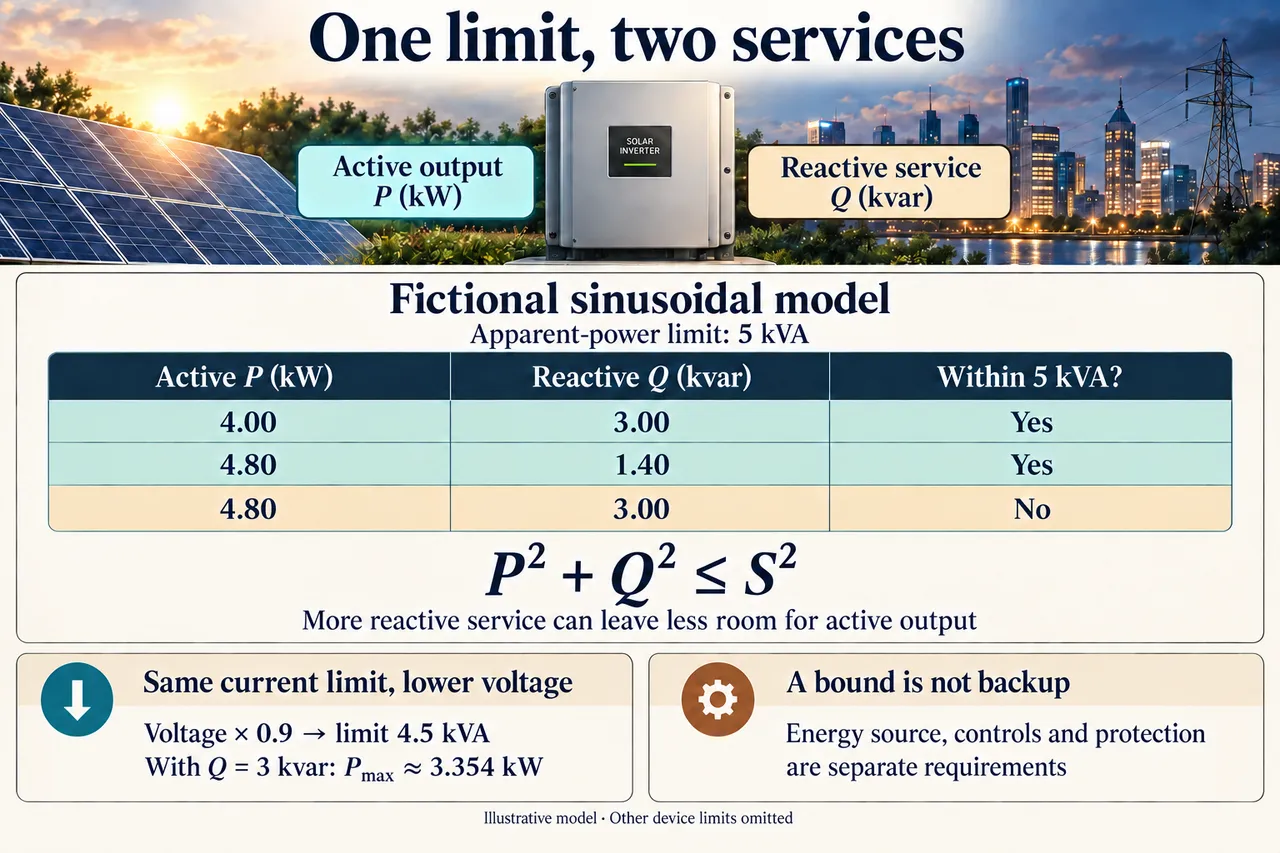
Original myAudience educational illustration. Image: illustration, not a documentary photograph. · myAudience educational illustration; fictional model, no certified rating or installation qualification implied.

One inverter limit, two services: active energy and reactive headroom

An inverter can provide active output and reactive service, but the two share electrical limits. Active power P is measured in watts and describes average energy transferred per second. Reactive power Q, measured in var, describes the phase-dependent exchange associated with electric and magnetic fields in the sinusoidal account. Apparent power S, measured in volt-amperes, combines the voltage and current magnitudes. Reactive exchange is not an extra stream of active energy and is not automatically converter heat. It can still increase current and associated resistive losses elsewhere in a network. This distinction matters when an inverter has enough solar energy available yet cannot simultaneously meet every requested electrical service.

For the original steady sinusoidal model, P = V_rms I_rms cos(phi) and Q = V_rms I_rms sin(phi), where phi is the voltage-current phase angle. Since cos squared plus sin squared equals one, P² + Q² = S², with S = V_rms I_rms. A stipulated current or apparent-power limit therefore bounds allowable combinations rather than setting independent maxima for P and Q. The simple relation assumes the declared single-phase sinusoidal boundary. Distorted waveforms, additional device restrictions or transient operation can require a fuller account. A circle drawn from one ideal limit is not the complete capability envelope of every physical inverter.

Suppose a fictional inverter has a 5 kVA apparent-power bound at nominal voltage and 4.8 kW of active output available after the modeled DC conversion stage. Request 3 kvar of reactive service and specify that this request takes priority for the exercise. The resulting active bound is sqrt(5²−3²)=4 kW, below the 4.8 kW available. The difference is 0.8 kW of active output foregone. If that same condition persists for exactly one hour, the active-energy difference is 0.8 kWh. Do not turn 3 kvar into 3 kWh of useful output or thermal loss: it is a different quantity with a different role in the sinusoidal current account.

Consider the alternative priority explicitly rather than pretend both requests fit. If active output remains 4.8 kW, the greatest reactive magnitude allowed by the same circle is sqrt(25−23.04)=1.4 kvar. That point meets the active request but fails the 3 kvar request. The requested pair would require sqrt(4.8²+3²)=5.660389 kVA before any other constraints are checked. Additional capacity could create headroom in this abstract model; it does not guarantee a voltage benefit, a lower lifetime cost or permission to use a particular control setting. Priority in these examples is a declared mathematical condition, not a recommendation to override approved network or device controls.

Voltage adds another important boundary. Suppose the actual restriction is a fixed RMS current limit that corresponds to 5 kVA at nominal voltage, and voltage falls to 0.9 of that value. With the same current allowance, V_rms I_max becomes 4.5 kVA. Keeping Q at 3 kvar leaves P no greater than sqrt(4.5²−3²)=3.354102 kW, so active output foregone rises to 1.445898 kW relative to 4.8 kW available. This does not say every device’s nameplate rating automatically changes with voltage in this way. It derives a conditional current-limited envelope; an actual device may have separate voltage, current, power, protection and control constraints that further restrict operation.

Reactive control can help manage a network voltage, but the amount of benefit depends on where the inverter connects and on the surrounding circuit. The cited historical interconnection report explains capability headroom and discusses interactions among controls. Its 2019 operating practices and adoption statements are not presented as current law. A small mathematical feasible point supplies neither a feeder model nor evidence that a chosen setting avoids oscillation or unwanted interactions. A more complete evaluation would define the measurement point, the network impedances, approved response rules and time-dependent disturbances, then validate the joint system rather than optimize one isolated number.

The useful services and their burdens should be made visible to affected people. Limiting active output can reduce a generator’s delivered energy while voltage support benefits other users; a decision may therefore need fair operating rules and a compensation method in addition to circuit calculations. More inverter capacity also entails materials, cost, maintenance and repair access. None of those values can be read from 5 kVA alone. A system that provides a feasible P-Q combination may still stop when the external grid disappears. Adequate energy supply, suitable grid-forming controls, safe isolation and protection, and sufficient load capacity are separate requirements for an intentional backup service.

The unfamiliar transfer uses a different apparent-power rating, available active output, reactive request and voltage change. First decide whether the requested point fits at nominal voltage; then recalculate the current-limited bound after the change. Keeping the original rating without checking V_rms I_max would conceal the new restriction. Image: illustration, not a documentary photograph. The two neutral labels identify services rather than directions of current flow, and the table depicts only the stipulated sinusoidal envelope. The plate is not a measured inverter specification, a control-setting instruction or evidence that a real system can supply isolated loads or stabilize a particular grid.

Worked example: At nominal voltage, assume a fictional 5 kVA apparent-power limit,4.8 kW available active output and a 3 kvar reactive request. Calculate the feasible active-priority and reactive-priority alternatives. Then lower voltage to 0.9 nominal at unchanged RMS current limit and retain the 3 kvar request. Explain the meaning and limits of each result.

Declare the sinusoidal steady boundary and units: P in kW, Q in kvar and S in kVA. The limit is one joint envelope, P²+Q²≤25, not permission to deliver 5 kW and 5 kvar together. Available 4.8 kW describes an active-output opportunity after conversion, rather than a new DC efficiency calculation. Squaring quantities expressed in the declared kilo-units gives consistent squared kilo-units. Combining watts with kilovolt-amperes without conversion would instead make a thousandfold unit error before any conclusion about capability was drawn.

Hold Q at 3 kvar for the stipulated reactive-priority case. P≤sqrt(25−9)=4 kW, so 4.8−4=0.8 kW of active output is foregone. For one hour, the active-energy difference is 0.8 kWh. The reactive quantity 3 kvar is not added to this energy balance as 3 kWh or converter heat. This is the positive active-output branch of the envelope. The negative reactive request of equal magnitude would leave the same mathematical active bound because Q is squared, although its network effect and approved control meaning could differ.

Hold P at 4.8 kW instead. Q≤sqrt(25−4.8²)=1.4 kvar. That meets the active request but not the required 3 kvar. The joint request requiresS=sqrt(4.8²+3²)=5.660389 kVA. A different priority rule cannot erase this mathematical conflict, and this exercise does not prescribe an operating control. Substitute the candidate pair back into the inequality: 23.04 plus 9 equals 32.04, exceeding 25. This independent substitution catches the common mistake of checking each request separately against five and declaring their combination acceptable.

Assume the binding limit is fixed RMS current. At voltage 0.9 nominal, apparent capability becomes 0.9×5=4.5 kVA. Keep Q=3 kvar: P≤sqrt(4.5²−3²)=sqrt(11.25)=3.354102 kW. Relative to 4.8 kW available, active curtailment is 1.445898 kW; sustaining the condition for one hour would forego the same numerical amount in kWh. The voltage factor changes the boundary before the square root is evaluated. Multiplying the nominal active result of four by 0.9 would give 3.6 kW, which would not preserve the unchanged three-kvar request and would exceed the correct joint limit.

Compare only matched boundaries. The 5 kVA and 4.5 kVA cases have different voltage conditions at the same current allowance. Do not label their difference an efficiency improvement or lost reactive heat. Actual individual P/Q, DC-bus, thermal, voltage, waveform and protection restrictions can narrow the ideal envelope. At fixed voltage, an increased apparent load generally requires increased RMS current in this model. A real conductor’s resistive dissipation depends on current squared and resistance; the apparent-power figure alone does not give that resistance or quantify the resulting heat.

Conclude what has and has not been established. The calculations identify incompatible requests and conditional headroom; they do not predict a network’s voltage response or certify a product. A feasible steady point also supplies no energy reserve, approved islanding, grid-forming controls or adequate backup load capacity. Those need distinct system evidence. Test a proposed conclusion by naming the missing evidence. Predicting voltage support requires a network model; estimating energy loss requires a duration or time series; assessing backup requires energy and control arrangements. The power triangle answers none of those additional questions by itself.

Answer: At the nominal 5 kVA bound, Q=3 kvar permits at mostP=4 kW, so 0.8 kW is foregone relative to 4.8 kW available. KeepingP=4.8 kW instead permits at mostQ=1.4 kvar and fails the 3 kvar request. The full pair requires 5.660389 kVA. At 0.9 nominal voltage with unchanged RMS current limit, S≤4.5 kVA and Q=3 leavesP≤3.354102 kW, with 1.445898 kW foregone. These are conditional sinusoidal bounds, not device efficiency, a voltage prediction, approved operating settings or backup-service certification.

Check your understanding: A different fictional inverter has a 6 kVA limit, 5.5 kW of available active output and a 2 kvar reactive request. Can both fit? Voltage then falls by 20% while maximum RMS current stays fixed. Find the new active-power bound with Q still 2 kvar. Why does a feasible operating point not prove islanded backup capability?

Answer: At nominal voltage the requested point requires sqrt(30.25 + 4) = 5.852350 kVA, below the 6 kVA bound. Reducing voltage by 20% with the same RMS current limit reduces the bound to 4.8 kVA. With Q fixed at 2 kvar, P ≤ sqrt(23.04 − 4) = 4.363485 kW, leaving 1.136515 kW of active output foregone. Backup additionally requires an adequate energy source, suitable grid-forming and isolation/protection arrangements, and sufficient load capacity; the steady power geometry proves none of those.

Why: Use a genuinely different requested point and voltage change. Apparent capability follows the declared voltage/current boundary, while reactive and active requests share the same envelope. Fit at nominal voltage does not prove fit after the change or establish the independent energy, control and protection conditions needed for isolated backup.