The same charge can deliver different useful energy

By How things work · myAudience

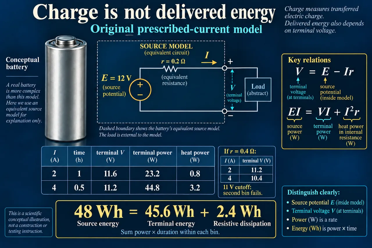
myAudience original rendered teaching illustration. Image: illustration, not a documentary photograph. · Operator-authored generated illustration; original scientific teaching model reviewed separately.

The same charge can deliver different useful energy

A battery’s chemical changes support electrical work, but the work reaching its terminals need not equal the energy released within the chosen source model. The earlier lesson separates electrons in the external circuit from ions in the cell. Here we ask a different question: why can a pack show a plausible voltage when idle yet fail to supply an intended load? OpenStax introduces a source with an electromotive force and an equivalent internal resistance. Despite its name, electromotive force is a voltage, not a mechanical force. We use that simple representation to construct an original accounting exercise, rather than reproduce a commercial lithium-ion cell’s full behaviour.

Draw the equivalent resistance inside the source boundary and the useful load outside it. During the declared discharge, terminal voltage is V = E − Ir, where E is the stipulated source voltage, I the prescribed discharge current and r the equivalent resistance. Multiplication by current gives EI = VI + I²r. The left side is the model’s source power; the right separates terminal electrical output and resistive dissipation. The resistor symbol is a mathematical stand-in for one loss contribution, not a claim that a discrete resistor can be found inside the cell. Electrochemical kinetics, changing composition, relaxation and temperature effects are omitted.

A prescribed-current load is an important assumption. In the original example it draws two amperes for one hour, then four amperes for half an hour. A fixed resistor would instead draw a current determined by its resistance together with the source; a regulated constant-power converter can draw more current as voltage falls. Those are different systems and cannot silently inherit the same numbers. We also stipulate an unchanging E of 12 V and r of 0.2 Ω throughout the bins. This is an invented short-profile surrogate, not a claim that a real battery maintains the same open-circuit potential across its whole state-of-charge range.

At two amperes, the internal drop is 2 × 0.2 = 0.4 V, so the load receives 11.6 V. Terminal power is 23.2 W, source power 24 W and the modeled resistive loss 0.8 W. At four amperes the drop becomes 0.8 V, terminal power 44.8 W, source power 48 W and loss 3.2 W. Doubling current quadruples this fixed-resistance loss term, while terminal output does not simply double because voltage also changes. A power figure is an instantaneous rate; the duration determines the associated energy. The second bin lasts half as long, which matters when comparing its energy with the first.

Integrate the two bins before comparing totals. Delivered charge is 2 × 1 + 4 × 0.5 = 4 Ah, or 14,400 C. Terminal electrical energy is 23.2 × 1 + 44.8 × 0.5 = 45.6 Wh. The model’s source energy is 24 × 1 + 48 × 0.5 = 48 Wh, and its resistive dissipation is 0.8 × 1 + 3.2 × 0.5 = 2.4 Wh. The account closes as 48 = 45.6 + 2.4 Wh. Multiplying all four ampere-hours by the 12 V source value produces the source-side estimate, not the terminal output. The difference follows from the declared boundaries rather than missing charge.

Change only equivalent resistance to 0.4 Ω, holding source voltage and prescribed current fixed. Terminal voltages become 11.2 and 10.4 V. The unconstrained calculation gives 43.2 Wh terminal energy and 4.8 Wh resistive loss, still closing the same 48 Wh source account. Now impose a fictional allowed terminal-voltage threshold of 11 V. The first bin meets it, but the second does not. Therefore 43.2 Wh is a counterfactual mathematical total for a profile that this threshold would reject. It is not a promise of permitted operation. A controller’s response after a threshold failure would need its own model; we do not invent continued operation, recovery or a reduced-current policy.

The changed resistance illustrates a limitation without diagnosing its cause. Comparing an idle voltage with a loaded voltage can reveal that a source representation needs a drop, but one measurement does not distinguish aging from temperature, state of charge, connectors or other losses. A real assessment needs a declared measurement point, compatible test conditions and appropriate equipment. Some energy stored in a cell may remain inaccessible to a particular load once a voltage or current limit binds. That is different from all remaining energy having been converted into heat. Neither an ampere-hour label nor our two-bin calculation measures the cell’s remaining lifetime or authorizes opening, rebuilding or improvising a charging system.

For the transfer, change source voltage, resistance, both current bins, their durations and the threshold; recompute rather than reuse the first answer. Then change resistance again and ask whether the full prescribed service remains allowed. A design comparison should consider the load’s actual requirements, competent repair, replacement cost, material recovery and the people who handle discarded cells. Those decisions require evidence beyond one calculated loss term. Image: illustration, not a documentary photograph. The conceptual equivalent-source diagram and energy table explain a model; they are not a physical cell cutaway, a wiring procedure, a measured specification or a safe battery-test instruction.

Worked example: A fictional source has constant 12 V emf and 0.2 Ω equivalent resistance. A prescribed load draws 2 A for 1 h, then 4 A for 0.5 h. Find charge, terminal energy and resistive dissipation. Change only resistance to 0.4 Ω and check an 11 V terminal cutoff.

Declare the source and terminal boundaries first. The source voltage E is fixed at 12 V, the equivalent resistance is 0.2 Ω, and the current profile is prescribed independently of terminal voltage. This model excludes changes in chemical state, auxiliaries and converter behaviour. Current multiplied by hours produces ampere-hours; multiplying it by voltage produces electrical power before duration is applied.

Calculate each terminal voltage rather than assign the source voltage to the load. The first bin has V = 12 − 2 × 0.2 = 11.6 V; the second has V = 12 − 4 × 0.2 = 11.2 V. Both are above the later stipulated 11 V cutoff in this original case. The voltage drop is inside the modeled source boundary.

Find rate quantities within each bin. Terminal powers are 11.6 × 2 = 23.2 W and 11.2 × 4 = 44.8 W. Source powers are 24 and 48 W; resistive losses I²r are 0.8 and 3.2 W. In each bin verify source power equals terminal power plus loss, which checks the algebra before integrating.

Apply the durations to every energy term consistently. Terminal energy is 23.2 × 1 + 44.8 × 0.5 = 45.6 Wh. Source energy is 24 × 1 + 48 × 0.5 = 48 Wh; resistive dissipation is 0.8 × 1 + 3.2 × 0.5 = 2.4 Wh. Charge is 4 Ah = 14,400 C. Check 48 = 45.6 + 2.4 Wh rather than adding ampere-hours directly to energy.

Change only resistance to 0.4 Ω. Voltages become 11.2 and 10.4 V, so unconstrained terminal energy is 11.2 × 2 × 1 + 10.4 × 4 × 0.5 = 43.2 Wh. Resistive dissipation doubles to 4.8 Wh because current is held fixed. The same 48 Wh source account closes, but this is not evidence that a real changing source preserves its voltage or prescribed load.

Apply the additional threshold to candidate operation. The second bin at 10.4 V violates the stipulated 11 V limit. Thus the full changed-resistance profile is inadmissible; its 43.2 Wh is not an allowed-service prediction. The original profile passes this particular voltage test, but that alone does not check real current ratings, temperature, protection, charging or lifetime. Name these missing conditions before drawing a product conclusion.

Answer: The original profile transfers 4 Ah, exports 45.6 Wh at the terminals and dissipates 2.4 Wh within the equivalent resistance, closing the 48 Wh modeled source account. Changing only resistance to 0.4 Ω gives an unconstrained 43.2 Wh terminal total and 4.8 Wh dissipation, but its second bin at 10.4 V fails the 11 V cutoff. The rejected profile cannot be reported as allowed service; controller response and other physical limits require further evidence.

Check your understanding: Use a 10 V source with 0.1 Ω resistance:1 A for 2 h, then 3 A for 1 h. Does it meet a 9.6 V cutoff, and how much terminal energy, loss and charge result? Change resistance to 0.2 Ω only; can the same full service still be claimed?

Answer: At 0.1 Ω, voltages 9.9/9.7 V meet 9.6 V. Charge is 5 Ah, terminal energy 19.8+29.1=48.9 Wh, resistive loss 0.2+0.9=1.1 Wh, and source energy 50 Wh. At 0.2 Ω, voltages 9.8/9.4 V fail the second threshold, so the full service is not permitted by this model. Equal prescribed charge is not proof of permitted delivered energy.

Why: The transfer changes every original input, then asks for a second boundary check. Integrate voltage times current, not charge alone; verify source energy equals output plus dissipation. A calculated candidate below cutoff cannot be relabeled as available useful service.