Round-trip efficiency needs a round trip

By How things work · myAudience

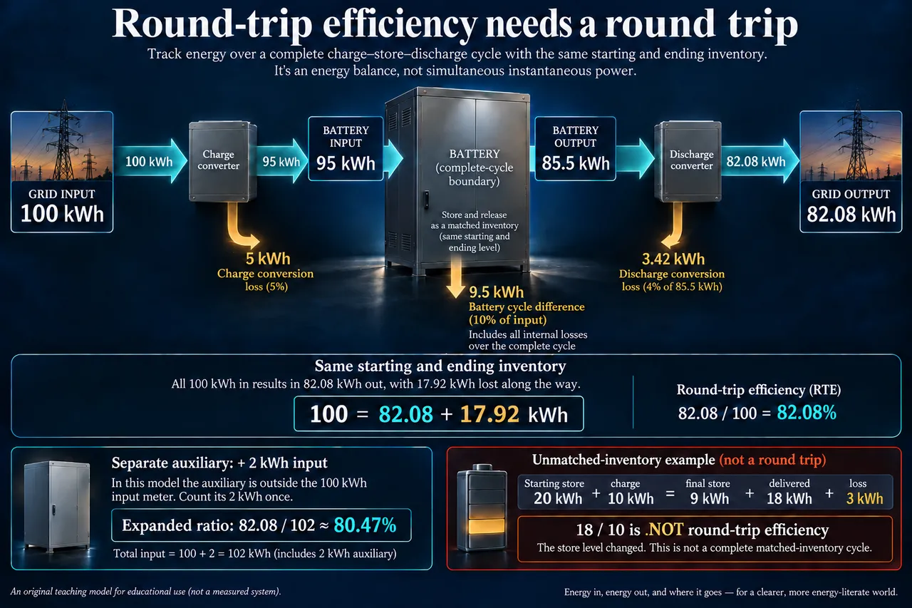
myAudience original rendered teaching illustration. Image: illustration, not a documentary photograph. · Operator-authored generated illustration; original scientific teaching model reviewed separately.

Round-trip efficiency needs a round trip

An energy-storage claim begins with its boundary. A cell terminal, a battery pack, a converter and a grid connection describe different places at which energy can be counted. A device can have a high efficiency at one of these boundaries while the complete service has additional losses. A round-trip ratio compares energy delivered with energy supplied over a suitable charging-and-discharging interval. It does not compare two convenient instantaneous power readings. The DOE-supported 2023 battery evaluation report stresses the need for charge and discharge records and attention to stored energy at the interval’s beginning and end. We build a separate original example to expose those distinctions.

First specify a complete cycle that returns the stored-energy inventory to its starting value. Charge-side conversion accepts 100 kWh from the grid and passes 95 kWh to the battery boundary. A stipulated aggregate battery-cycle ratio of 0.90 then gives 85.5 kWh from that boundary during discharge. A discharge-side converter delivers 96% of that amount: 82.08 kWh to the grid-side output. Multiplying the three ratios gives 0.95 × 0.90 × 0.96 = 0.8208. The battery’s 90% and the complete path’s 82.08% are both conditional results, but they refer to different boundaries and cannot be substituted for each other.

Track the differences as well as the ratios. The charge-side converter loses 5 kWh between its input and output. The battery-cycle difference is 95 − 85.5 = 9.5 kWh; the discharge-side converter difference is 85.5 − 82.08 = 3.42 kWh. These sum to 17.92 kWh, matching 100 − 82.08. We have deliberately used an aggregate battery-cycle ratio without assigning its loss to charging, discharging or standby individually. Infinitely many distributions could produce the same aggregate number. Dividing that loss equally between the two legs would introduce another assumption rather than discover a measured fact about chemistry or thermal behaviour.

Now widen the input boundary to include a separate auxiliary that consumes 2 kWh during this cycle. By stipulation that auxiliary was not already included in the original 100 kWh meter total. The expanded input is therefore 102 kWh, and the expanded delivered-to-input ratio is 82.08/102, approximately 80.47%. The additional energy could be part of operating the wider installation even though it never appears as battery output. If the original meter already included it, adding it again would double count. Always say where each meter sits and what its total contains before comparing storage systems, especially when one efficiency excludes support equipment and another includes it.

A different interval can produce a surprising output/input ratio without producing new energy. Start with 20 kWh of stored energy. Supply 10 kWh to a fictional charging boundary that stores 90%, adding 9 kWh and losing 1 kWh. Later withdraw 20 kWh from the inventory; a discharge process delivers 90%, or 18 kWh, and loses 2 kWh. The final stored energy is 20 + 9 − 20 = 9 kWh. The complete account is 20 + 10 = 9 + 18 + 3 kWh. Yet a naive meter-only ratio is 18/10 = 180%. The installation used part of its initial inventory; that unmatched interval is not a complete round-trip test.

The inventory exercise also explains why a battery cannot be evaluated as though every hour is independent. A previous hour may change what can be supplied in the next one. Beginning and ending state-of-charge estimates help interpret measurements, but a percentage is not automatically an exact stored-energy reading across chemistry, aging and temperature. Our 20 and 9 kWh inventories are stipulated directly, so no uncertain SOC-to-energy conversion is hidden in the arithmetic. A practical estimate needs appropriate calibration and matching conditions. Large throughput can reduce the relative effect of endpoint differences, but it cannot repair missing measurements or make an inconsistent boundary become consistent.

Keep gross charge and discharge separate when collecting an account. A signed net-flow total can conceal energy moving in both directions within an interval: equal charging and discharging contributions may sum to zero although both processes occurred. The evaluation report also cautions that zero measured flow alone cannot distinguish an unavailable system from one that was simply not asked to operate. Dispatch records, device responses and measurement quality are additional evidence. A calculated ratio should therefore be accompanied by interval, boundary, operating conditions and uncertainty. Do not present an idle day as proof of a failure, or an incomplete energy record as a certified efficiency measurement.

The transfer is a design-reasoning test, not a search for the largest reported percentage. Explain the apparent 180% before choosing which records need improvement. Compare dependable delivered service, required charging energy, repair access, replacement frequency and the conditions under which users actually need power. A high ratio by itself says nothing about the production source’s emissions, the battery’s material supply chain or an installation’s safe outage operation. Image: illustration, not a documentary photograph. The large plate’s arrows represent integrated energy through declared cycle boundaries, not instantaneous simultaneous power or a wiring design. The separate inventory inset must not be mistaken for another matched cycle.

Worked example: A matched-inventory cycle takes 100 kWh grid input. Charging conversion is 95%, the aggregate battery-cycle ratio 90%, and discharge conversion 96%. Compute delivered energy and all three differences. Then widen the input boundary with an additional 2 kWh auxiliary outside the original meter.

Declare a cycle with the same initial and final stored-energy inventory. Without this condition, output/input can include energy borrowed from the starting store or energy left for later use. The input and output meters in this exercise sit at grid-side boundaries. The aggregate battery-cycle ratio applies between battery-terminal charge and discharge totals; it is not a single-direction charging factor.

Pass energy through the first boundary: 100 × 0.95 = 95 kWh reaches the battery charge boundary. The difference of 5 kWh belongs to the charging-conversion stage. It is already reflected in the reduced 95 kWh, so it must not be subtracted again when applying the battery-cycle ratio. All numbers describe energy integrated over the declared interval, not ratings in kilowatts.

Apply the aggregate battery-cycle ratio to its own input. The battery discharge total is 95 × 0.90 = 85.5 kWh. Its 9.5 kWh cycle difference is not known to occur entirely during charging or discharge. The assumed ratio contains no unique decomposition of chemical, resistive or standby contributions. Naming those mechanisms would require additional measurements or another explicitly stated model.

Apply discharge conversion once: 85.5 × 0.96 = 82.08 kWh reaches the grid-side output. The difference for this stage is 3.42 kWh. Check the entire account using 5 + 9.5 + 3.42 = 17.92 kWh, then 82.08 + 17.92 = 100 kWh. Matching beginning and ending inventory allows this closed full-cycle comparison.

Compare like boundaries. Battery-terminal cycle efficiency is 85.5/95 = 0.90, whereas grid-side cycle efficiency is 82.08/100 = 0.8208, or 82.08%. Multiplication of the three ratios reproduces the latter. Neither is an efficiency of every real battery or converter; these are original stipulated constants chosen to make the boundaries visible. A different load, temperature or interval would require suitable evidence.

Expand only the input boundary to include the separate auxiliary. By assumption it consumes an additional 2 kWh outside the first meter; total input is 102 kWh. Delivered output remains 82.08 kWh, so the expanded ratio is approximately 80.47%. The widened difference is 19.92 kWh. If the initial meter had already included auxiliaries, this addition would be invalid double counting rather than a more complete account.

Answer: The chain delivers 82.08 kWh. Stage differences 5,9.5 and 3.42 kWh total 17.92 kWh, closing 100=82.08+17.92. The battery-terminal cycle ratio 90% and grid-side 82.08% use different boundaries. Adding a genuinely separate 2 kWh auxiliary widens input to 102 kWh and reduces the complete ratio to about 80.47%. These stipulated matched-inventory results do not determine chemistry-specific losses or guarantee measured annual performance.

Check your understanding: Start with 20 kWh stored. A 10 kWh charging input adds 9 kWh; withdrawing 20 kWh later delivers 18 kWh. What inventory remains, how much is lost, and does 18/10 demonstrate 180% round-trip efficiency?

Answer: Stored energy ends at 20+9−20=9 kWh. Charging loss 1 kWh plus discharge loss 2 kWh totals 3 kWh. The balance is 20+10=9+18+3. The 18/10 ratio uses an interval whose inventory falls 11 kWh, so it is not matched-cycle efficiency and provides no free energy. Obtain matched endpoints or an appropriately evidenced inventory account before reporting a round-trip result.

Why: The unfamiliar transfer changes from a closed cycle to an interval drawing on starting energy. Accounting for inventory removes the apparent paradox. Summing only the two meter readings cannot distinguish energy supplied during this interval from energy stored beforehand; a useful efficiency claim must preserve its boundary and endpoint conditions.