An image takes many listens: ultrasound acquisition time and sampling tradeoffs

By How things work · myAudience

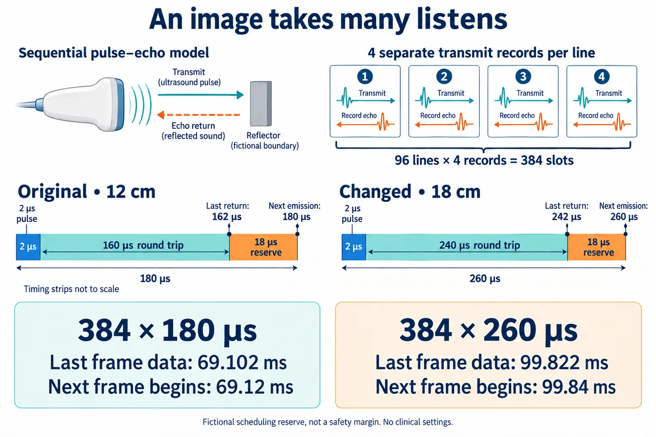
Image: illustration, not a documentary photograph. Fictional sequential acquisition schedule; a supplied reserve separates the final echo from the next emission, without prescribing clinical settings. · Operator-authored generated teaching illustration; scientific concept/model review retained separately.

An image takes many listens: ultrasound acquisition time and sampling tradeoffs

A moving ultrasound image is assembled from measurements made over time. A scan line describes one direction through the region being represented, while a frame combines information from many such directions. Within one direction, an instrument emits a short acoustic pulse and records returning echoes. The carrier oscillations inside that pulse, the number of separate pulse emissions and the number of completed frames are different counts. Confusing them can make a fast-sounding frequency label stand in for an image rate that it does not determine. Our earlier lesson explained how a returning echo can be assigned a distance using an assumed sound speed. Here the question changes: how long does a sequence of records take, and what must be sacrificed when a specified time budget is too short? We use a fictional sequential instrument to expose those dependencies. Its supplied values describe an educational schedule, not a scanner setting, clinical examination or measured product performance. Knowing exactly what is counted allows us to explain a limit without pretending that the calculation evaluates a person's health.

Start with one emission and identify its beginning and end. In the supplied uniform medium, the leading edge travels to the deepest included boundary and back in 2D/c seconds, where D is maximum depth in metres and c is the assumed speed in metres per second. A pulse lasts a finite time. Its last part leaves after the first part, so the final deepest return occurs one pulse duration later than the leading-edge return. We then reserve an additional fictional interval before the next emission. The leading-edge-to-leading-edge slot is therefore pulse duration plus deepest round-trip time plus this reserve. The reserve is part of the exercise's scheduling boundary; it is not a validated safety margin. We assume one sequential acquisition at a time, a fixed speed and no unspecified processing or steering overhead. Those assumptions deliberately simplify the schedule. They do not state that real echoes end sharply at this depth, that all tissues have the same speed, or that other acquisition architectures must use this exact timing.

A composite scan line can require more than one separately transmitted record. In this exercise there are four transmit focal-zone acquisitions for each line. Each record consumes its own emission-and-listening slot; combining them afterwards does not recover the time already spent acquiring them. The IAEA's 2014 teaching account explains the corresponding tradeoff between repeated transmit focusing and frame rate. Receive focusing is a different operation: recorded signals can be combined using changing delays during reconstruction without inherently requiring another acoustic emission. This distinction does not make receive processing free in an actual instrument, and it does not promise that one receive operation produces the same result as four transmitted records. Nor do four records automatically mean four independent statistical averages. We specifically count separate transmissions serving a supplied composite-line model. Keeping physical acquisition separate from reconstruction helps identify which proposed change could reduce the schedule and which would merely change later computation. The model supplies no comparison of clinical image quality between focusing methods.

For the original case, the maximum depth is 12 cm, or 0.12 m, and the assumed sound speed is 1500 m/s. The leading-edge round trip is 160 microseconds. A two-microsecond pulse places the final deepest return at 162 microseconds; the additional 18-microsecond reserve makes the slot 180 microseconds. Ninety-six lines would consume 17.28 milliseconds with one acquisition per line. Four separate acquisitions per line instead require 384 slots and a sustained frame-cycle budget of 69.12 milliseconds. Its inverse is about 14.4676 frames per second. The final data from the last record arrive at 69.102 milliseconds, 18 microseconds before that cycle boundary. This distinction matters: waiting for the required reserve before beginning the next frame is not the same event as receiving the final echo. We count the reserve after every record, including the last, because the question asks about repeating this schedule. A carrier frequency measured in megahertz cannot substitute for any of these frame-cycle calculations.

A target of 25 frames per second permits a repeating cycle of 40 milliseconds. The original four-record, 96-line schedule therefore misses the supplied target. If only the line count may change, each line still costs four 180-microsecond slots, or 0.72 milliseconds. Dividing the available time by that cost gives a continuous bound of 55.555… lines. A line count must be a whole number, so the greatest allowed count is 55, not a rounded-up 56. Direct checks establish the boundary: 55 lines take 39.60 milliseconds, whereas 56 take 40.32 milliseconds. This is a timing result with an explicit permitted change. It does not show that the original coverage or detail survives. Over the same span, fewer line positions mean wider spacing; retaining spacing instead could require a narrower span. A useful design argument states that tradeoff openly. It cannot turn a deadline calculation into evidence that the resulting image is sufficient for diagnosis or that an operator should select these values.

Now change the maximum depth to 18 cm while keeping the other supplied assumptions. The leading-edge round trip becomes 240 microseconds, and the pulse's final part returns at 242 microseconds. Including the same fictional reserve gives a 260-microsecond slot. Retaining the old 180-microsecond slot would start a new emission before the final modeled deepest return from the previous one. It would therefore violate this exercise's nonoverlapping acquisition boundary. That conclusion applies to this specified sequential model, not to every possible coded, parallel or overlapping method. With 96 lines and four records per line, the sustained cycle becomes 99.84 milliseconds, about 10.0160 frames per second. Its last deepest return arrives at 99.822 milliseconds. Depth has increased by one half, but slot time has not increased by exactly one half because the fixed pulse duration and reserve remain additive terms. Following the full equation, rather than scaling only the distance, preserves both the physical reasoning and the stated boundary.

The changed target is 15 frames per second, giving a cycle allowance of 1/15 second, approximately 66.6667 milliseconds. Each four-acquisition line now costs 1.04 milliseconds. The greatest integer count that fits is 64: those lines require 66.56 milliseconds, while 65 require 67.60 milliseconds and miss. To examine what this buys, suppose the same fictional line positions span 38 mm and include both endpoints. Ninety-six positions make 95 intervals, giving 0.4 mm spacing. Sixty-four positions make 63 intervals, giving 38/63 mm, approximately 0.60317 mm. Count intervals rather than dividing by the number of positions. The changed arrangement is coarser across that fixed span. This spacing is not itself the instrument's lateral resolution: beam properties, reconstruction and other factors also matter. The arithmetic demonstrates a timing-versus-sampling tradeoff, while leaving open whether the sampling is adequate for any particular purpose. Neither passing the cycle deadline nor preserving an endpoint span answers that separate question.

A transparent acquisition budget helps learners discuss responsiveness without treating speed as the only value. A longer cycle can make updates less frequent; fewer lines can weaken spatial sampling or reduce the represented span. More complex acquisition and processing may change those relationships, but they need their own stated model and evidence. Uniform sound speed, omitted overhead and a fixed reserve are assumptions to revisit, not guarantees built into nature. They also leave questions of access, operator training, interpretation and equipment suitability unresolved. NIH describes ultrasound's pulse-and-echo basis, while FDA explains that nonionizing ultrasound still introduces energy and can have biological effects. Those facts support appropriate professional use, not a safe-exposure prescription derived from this exercise. We provide no scanning procedure, calibration instructions, clinical diagnosis, equipment rating or approval. The worked answers establish only the supplied counting and timing consequences. Practical competence, assessment coverage and any claim about real medical adequacy remain open, with the earlier mechanism lesson and its artwork preserved.

Worked example: A fictional sequential instrument has maximum uniform depth 12 cm and assumed sound speed 1500 m/s. Every pulse lasts 2 µs, followed after its final deepest return by a supplied 18 µs reserve. It acquires 96 lines with four separate transmit focal-zone acquisitions per line. Ignore unspecified processing, steering and switching overhead; allow no acquisition parallelism. Find the slot, sustained frame-cycle budget, last-data arrival and repeating frame rate. Test a 25 frames/s target and find the greatest integer line count that meets it when only line count can change.

Convert the original depth before using the speed: 12 cm = 0.12 m. The sound must travel out and back, so the leading-edge path is 0.24 m. Dividing by the assumed 1500 m/s gives 0.000160 s, or 160 µs. This value describes the leading-edge return from the deepest modeled boundary. It does not include the pulse's finite duration or the supplied reserve, and it does not measure the complete frame.

The pulse lasts 2 µs, so its final part returns at 160 + 2 = 162 µs after the leading edge was emitted. Add the supplied 18 µs reserve to obtain a 180 µs leading-edge-to-leading-edge slot. Keep the quantities separate: 160 µs is leading-edge travel, 162 µs is final modeled return, and 180 µs is the next permitted emission under this fictional sequential schedule. The reserve is not an approved safety margin.

Count physical acquisitions rather than carrier oscillations. With one acquisition on each of 96 lines, there would be 96 slots, taking 96 × 180 µs = 17.28 ms. The specified four separate transmit focal-zone records require 96 × 4 = 384 slots instead. Their sustained cycle takes 384 × 180 µs = 69.12 ms. Reconstruction can combine the records later, but cannot remove the time spent emitting and listening for them.

Invert the sustained cycle in seconds: 1/0.06912 = 15625/1080 ≈ 14.4676 frames/s. The last deepest return occurs 18 µs before the next-frame boundary, at 69.102 ms; it is not the repeating cycle duration. A target of 25 frames/s permits 1/25 s = 40 ms, so 69.12 ms misses it. Compare periods or rates consistently rather than comparing a duration directly with a frame count.

For the permitted line-count change, solve N × 4 × 180 µs ≤ 40 ms. The continuous bound is 500/9 = 55.555… lines, so its integer floor is 55. Verify both neighboring counts: 55 × 0.72 ms = 39.60 ms meets the allowance, while 56 × 0.72 ms = 40.32 ms misses it. The second check proves maximality rather than merely finding one count that happens to pass.

Report the complete conditional result: 180 µs slots, 69.12 ms sustained cycles for the original 96-line arrangement, and at most 55 lines for the supplied 25 frames/s target. The last-data and next-frame events remain distinct. Reducing line count changes sampling or coverage, so timing success alone cannot establish unchanged detail or diagnostic adequacy. The calculation supplies neither scanning instructions nor a clinical safety or equipment-performance rating.

Answer: The leading-edge round trip is 160 µs and final pulse-part return is 162 µs, giving a 180 µs slot including the supplied reserve. The 384 acquisitions produce a 69.12 ms sustained cycle, with final data at 69.102 ms and about 14.4676 repeating frames/s. The 25 frames/s allowance is 40 ms, so the original schedule misses. At most 55 lines fit: 39.60 ms meets, while 56 lines take 40.32 ms and miss. These results establish only the fictional timing boundary, not safe operation, diagnostic quality or measured scanner performance.

Check your understanding: Change maximum depth to 18 cm while retaining the assumed speed, pulse duration, reserve and four separate acquisitions per line. Require 15 repeating frames/s. Derive the slot, 96-line sustained cycle and final-data arrival. Find the greatest integer line count that fits, checking the next count. Compare spacing across an unchanged fictional 38 mm span that includes both endpoints. Does retaining the old 180 µs slot satisfy the same model, and does the passing line count prove clinically adequate sampling?

Answer: The leading-edge round trip is 2 × 0.18/1500 = 240 µs; the final pulse-part return is 242 µs. Adding the reserve gives a 260 µs slot. For 96 lines, 384 slots take 99.84 ms, with final data at 99.822 ms. The repeating rate is 3125/312 ≈ 10.0160 frames/s, below 15. The allowance is 1/15 s ≈ 66.6667 ms. Each four-record line takes 1.04 ms; the floor of the continuous bound 2500/39 ≈ 64.1026 is 64. Sixty-four lines take 66.56 ms and meet; 65 take 67.60 ms and miss. Original endpoint spacing is 38/95 = 0.4 mm; changed spacing is 38/63 ≈ 0.60317 mm. The old 180 µs slot begins another emission before the modeled 242 µs final return, so it does not meet the same nonoverlapping boundary. Coarser spacing is not proof of adequate lateral resolution or diagnosis, and no safe scan protocol follows.

Why: The changed calculation recomputes the distance-dependent round trip while preserving the fixed pulse and reserve terms. The sustained cycle includes the reserve after every acquisition, including the last; earliest final-data arrival is therefore 18 µs earlier, not a different frame-rate budget. Taking an integer floor and checking both 64 and 65 proves the greatest feasible count under the supplied rule. Endpoint positions create one fewer interval than positions. Separate timing, sampling, reconstruction and biological-effects questions prevent a passing arithmetic result from being mistaken for clinical or equipment approval.