Atoms spread, not march: diffusion distance and the time budget
By How things work · myAudience
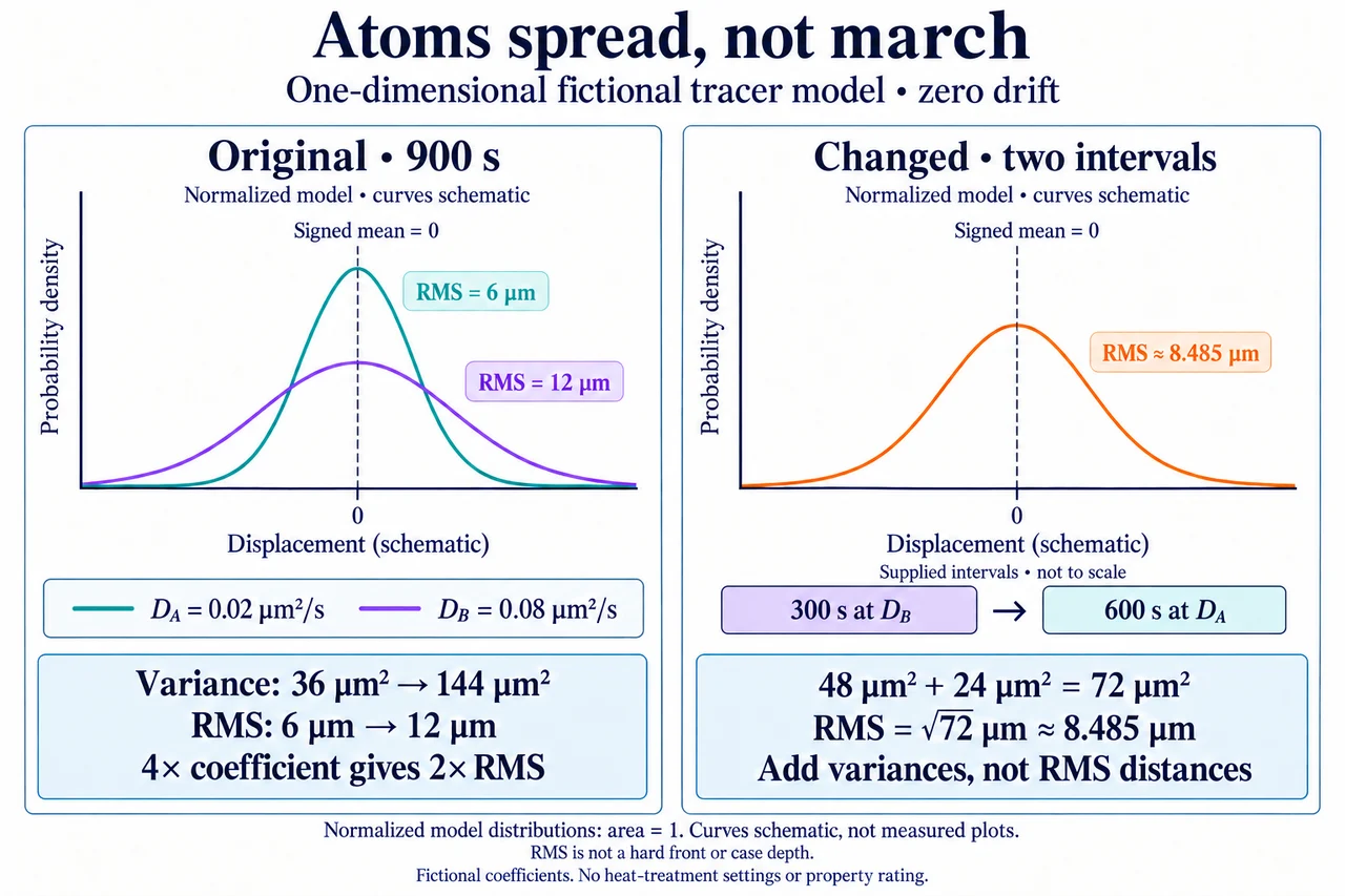
Image: illustration, not a documentary photograph. Fictional one-dimensional tracer spread; RMS displacement is a statistical width, not a hard front, case depth or heat-treatment prescription. · Operator-authored generated teaching illustration; scientific concept/model review retained separately.
Atoms spread, not march: diffusion distance and the time budget
A carbon balance can tell us how much carbon a closed sample contains, but it cannot tell us how quickly carbon redistributes. The earlier heat-treatment lesson kept that inventory consistent between a matrix and a carbide-rich phase. This lesson asks a different question: what does a supplied transport model predict about the spread of an initially localized collection of tracers? Diffusion concerns mass transport; it is not simply another name for heat flowing through a solid. Different species can have different mobilities, and a changing microstructure can create reactions, traps or alternative pathways that a simple transport equation omits. The Cambridge account of tempered martensite gives context for carbon redistribution and precipitation, while also showing why a single distance statistic cannot describe the whole transformation. We will use fictional coefficients without assigning them to an alloy, temperature or treatment process. The purpose is to make the consequences of a carefully stated mathematical boundary understandable, not to suggest a procedure for preparing a real component.
Imagine many tagged particles initially concentrated around a reference position that we call x = 0. Individual particles can move in either direction along the chosen coordinate. In a symmetric model with no drift, the signed average displacement remains zero because positive and negative displacements balance. That does not mean that every particle stays at its starting point. Squaring each displacement before averaging avoids cancellation and measures the spread. Taking the square root of that average gives the root-mean-square, or RMS, displacement. It is an ensemble statistic, not the itinerary of a particular atom. It is also different from the average absolute displacement, despite both having units of length. These distinctions matter when someone says that atoms have travelled a certain distance: the phrase could refer to a mean, a spread, an extreme value or a concentration threshold. A defensible calculation names the statistic before interpreting it, and avoids converting a statistical width into a guaranteed reach for all particles.
Our boundary is an effectively infinite, homogeneous, one-dimensional medium with zero drift, no reaction or trapping, and a spatially uniform positive diffusion coefficient D. The collection begins localized at the reference position. MIT's continuum teaching derives a normalized Gaussian distribution for this boundary and a mean-square displacement of 2Dt when D is constant. Normalization means that the total tracer population is conserved while its distribution spreads. In SI units, D is measured in square metres per second; multiplying by time produces square metres, and the square root returns metres. The distribution has no sharp advancing edge. Its RMS width is neither a maximum displacement nor the depth at which a chosen concentration is reached. A three-dimensional total-displacement calculation would use a different dimensional factor; we deliberately follow one coordinate. Finite surfaces, concentration-dependent coefficients, chemical reactions and evolving phases would require another model. The equation is useful precisely because its assumptions and its limited interpretation are explicit.
Choose a fictional coefficient D_A = 2 × 10⁻¹⁴ m²/s and an elapsed time of 900 s. Since one square metre contains 10¹² square micrometres, this coefficient is 0.02 µm²/s. The variance is then 2 × 0.02 × 900 = 36 µm², giving an RMS displacement of 6 µm. At the same elapsed time, a second supplied coefficient D_B = 8 × 10⁻¹⁴ m²/s, or 0.08 µm²/s, gives 144 µm² and an RMS displacement of 12 µm. The coefficient increases fourfold, but the RMS increases only twofold because of the square root. Both cases still have a signed mean displacement of zero. These values are original teaching inputs, not measured diffusion coefficients for carbon in a named steel. Neither case establishes a particular concentration profile near a real surface, the size of a precipitate, a hardness result or the acceptable condition of a manufactured part. The comparison concerns transport statistics under declared assumptions, rather than a ranking of commercial materials.
The same relationship can be read backwards. To obtain an RMS displacement of 12 µm at D_A, the required variance is 144 µm². Dividing by the variance growth rate, 2D_A = 0.04 µm²/s, gives 3600 s. This is four times the original 900 s for twice the original RMS displacement. The general scaling at fixed D is time proportional to the square of the requested RMS distance. It is not constant-speed motion, where twice the distance would take twice the time. A selected RMS target is a criterion for this exercise, not a threshold known to produce an approved microstructure. Real diffusion can accompany precipitation, recovery or changes in phase composition, and those processes require their own thermodynamic, kinetic and observational evidence. Treating the inverse equation as a sufficient heat-treatment schedule would silently add conclusions absent from the data. We therefore keep the fictional statistical criterion separate from any practical material-processing decision.
A changed problem makes the accounting more demanding by allowing D to vary with time while remaining uniform in space. For this same infinite-line, zero-drift boundary, the diffusion equation gives a second-moment growth rate of 2D(t). Integration over supplied intervals therefore adds their variance contributions, not their RMS lengths. Use D_B for 300 s and D_A for 600 s. The two contributions are 48 µm² and 24 µm², making 72 µm² in total. The RMS is √72 µm, or 6√2 µm, approximately 8.485 µm. Adding the individual square-root distances would describe neither this distribution nor this moment balance. Equally, averaging the two coefficients by counting two stages ignores their unequal durations. Their time-weighted coefficient over 900 s is 0.04 µm²/s, rather than the unweighted 0.05 µm²/s. The stage labels identify hypothetical coefficient intervals; they do not represent specified heating temperatures or an operating recipe. A model without precipitation cannot infer carbide formation merely from a larger integrated variance.
Suppose the changed statistical target is an RMS displacement of 9 µm within a total allowance of 1200 s, and only the final D_A interval may be extended. The target variance is 81 µm². The existing two intervals supply 72 µm², leaving 9 µm² to add. At a variance growth rate of 0.04 µm²/s, this needs another 225 s, for a total of 1125 s. That meets the supplied allowance. Using the full 1200 s instead extends the final interval by 300 s, making 84 µm² and an RMS of approximately 9.165 µm. Reversing the same two supplied coefficient-duration pairs leaves their integrated sum unchanged under this model. It does not prove that reversing real treatment stages gives the same material. When phases, trapping, interfaces or reactions evolve, the assumptions can fail and order can matter. The mathematical result establishes feasibility for a stated variance target, while identifying exactly why a stronger engineering claim would be unsupported.
A useful materials decision combines transport literacy with evidence beyond one favourable number. MIT's solid-state teaching emphasizes how atomic arrangement and conditions affect diffusion; bulk, surface and grain-boundary paths need not behave alike. An observed spread can also reflect measurement geometry or boundaries that our infinite-medium exercise excludes. Before connecting transport to service performance, ask which species and phases are present, how the starting state was characterized, and whether the relevant hardness, toughness, fatigue and corrosion behaviour were actually tested. Worker protection, energy use, traceability and the cost of failures also belong in a responsible comparison. Faster redistribution is not automatically a better product, and a predicted statistical width is not a qualification certificate. This lesson provides no alloy recipe, temperature, equipment control, heat-treatment instruction or dangerous handling procedure. The existing mechanism and artwork remain intact; these original calculations add a bounded explanation of kinetics. Full assessment, practical competence and safe-component claims remain open.
Worked example: A supplied fictional localized tracer ensemble diffuses along one coordinate in an effectively infinite homogeneous medium, with zero drift and no reactions or trapping. Compare its RMS displacement after 900 s at D_A = 2 × 10⁻¹⁴ m²/s and D_B = 8 × 10⁻¹⁴ m²/s. Find the time for a 12 µm RMS target at D_A. Explain the signed mean, units, scaling and why these results do not specify case depth or hardness.
Define the quantity before calculating it. For the supplied localized ensemble, let each displacement be measured from its initial reference along one coordinate. Zero drift and symmetry give a signed mean of zero, while the mean-square displacement is 2Dt. RMS means the square root of that second moment. We assume a homogeneous effectively infinite medium without reactions or trapping; no surface concentration threshold or material property is being predicted.
Convert the supplied coefficients without mixing linear and squared units. One metre is 10⁶ µm, so one square metre is 10¹² µm². Therefore D_A = 2 × 10⁻¹⁴ m²/s becomes 0.02 µm²/s, and D_B becomes 0.08 µm²/s. The variance rate is twice the coefficient in this one-dimensional model. Multiplication by seconds gives µm², not µm, until the final square root is taken.
Calculate the first case at 900 s: mean-square displacement is 2 × 0.02 × 900 = 36 µm². Its square root is 6 µm. A zero signed mean remains consistent with this nonzero spread, because the squared displacements do not cancel. The result does not say that every particle has moved exactly 6 µm or that no particle lies farther from the reference point.
At the same 900 s, D_B gives 2 × 0.08 × 900 = 144 µm² and an RMS displacement of 12 µm. Comparing like quantities, the variance is four times the first value while RMS is twice the first value. Do not compare a squared distance directly with a distance, or interpret the difference as a known increase in case depth, hardness or a finished component's quality.
Invert the first-case equation for a 12 µm RMS target. Square the target to obtain 144 µm², then divide by 2D_A = 0.04 µm²/s. The answer is 3600 s. Check it by substitution: 0.04 × 3600 = 144 µm², whose square root is 12 µm. Doubling the original 6 µm RMS target therefore requires four times its 900 s at fixed D_A.
Report both numerical results and their boundary: 6 versus 12 µm RMS after 900 s, and 3600 s for 12 µm RMS at D_A. These are ensemble spreads under supplied fictional coefficients, with signed mean zero. A concentration-threshold depth would require a different initial and boundary-value problem. Material transformation and qualification additionally require evidence absent here. No real treatment schedule, safe operating condition or component approval follows from the calculations.
Answer: At D_A, mean-square displacement is 36 µm² and RMS is 6 µm; at D_B, they are 144 µm² and 12 µm. A 12 µm RMS target at D_A requires 3600 s, four times 900 s for twice the original RMS. The signed mean remains zero in both cases. The fictional ensemble model predicts spread, not a maximum reach, surface threshold, hardening result or real treatment qualification.
Check your understanding: Retain the same infinite-line, spatially uniform, zero-drift, no-reaction boundary, but supply D_B for 300 s followed by D_A for 600 s. Derive the RMS displacement. A 9 µm RMS target must be reached within 1200 s total; only the final D_A interval may be extended. Find the extra and total time, and check the RMS at the full allowance. Would reversing the same coefficient-duration pairs leave the model result unchanged, and would that establish order-independent real heat-treatment properties?
Answer: For a time-dependent spatially uniform D, the second moment grows as 2D(t); integrate to add 2D_i t_i. The first interval contributes 2 × 0.08 × 300 = 48 µm², and the second contributes 2 × 0.02 × 600 = 24 µm². Total variance is 72 µm², giving RMS √72 = 6√2 ≈ 8.485 µm. The 9 µm target requires 81 µm², so 9 µm² remains. At 2D_A = 0.04 µm²/s this takes 225 s extra, giving 1125 s total, within 1200 s. At the full allowance, the final D_A interval is 900 s; total variance is 48 + 36 = 84 µm², giving RMS √84 ≈ 9.165 µm. Reversing the same supplied pairs preserves their integrated sum under this model. It does not establish that actual phase evolution, trapping, concentration-dependent transport or reactions are order-independent, nor that any hardness, safety or component qualification target is met.
Why: The second-moment relation follows by integrating the diffusion equation against x², with conserved normalization and decaying infinite-line boundary terms. It gives d⟨x²⟩/dt = 2D(t) for the stated uniform coefficient and zero-drift boundary. Contributions add as variances, not RMS distances. The time-weighted D over the original 900 s is (0.08 × 300 + 0.02 × 600)/900 = 0.04 µm²/s; the unweighted two-stage average 0.05 µm²/s is wrong for unequal durations. Squaring the target before solving and checking the full allowance keeps units and the permitted extension explicit. These are fictional transport statistics, not measured heat-treatment settings.