Rational powers: keep the domain when finding a tangent

By UK A Level Mathematics · independent study · myAudience

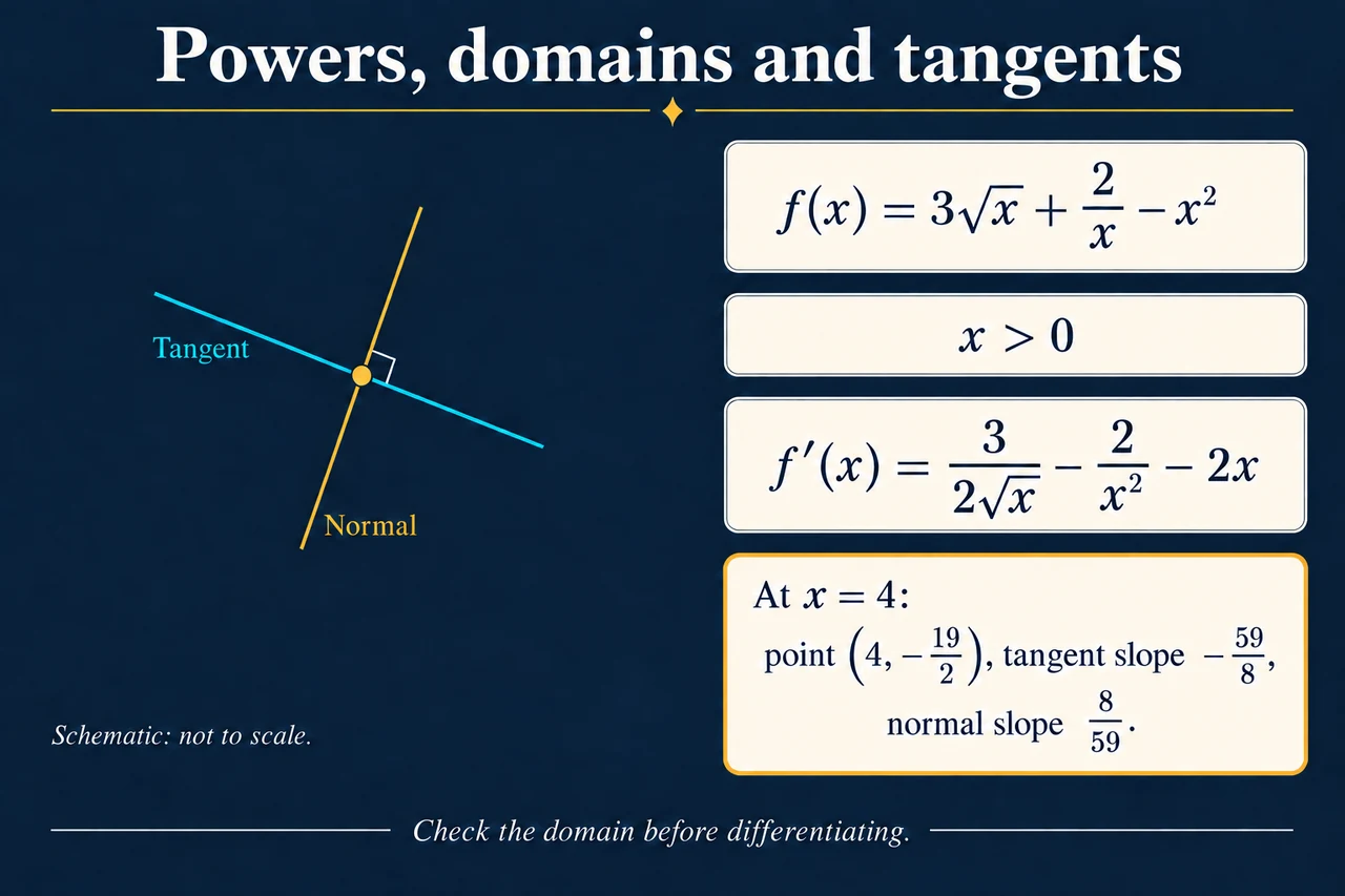
Image: illustration, not a documentary photograph. Conceptual point-and-line construction; original curve is intentionally omitted. No calibrated function graph is implied. · Original generated project artwork; no source textbook or exam-board figures reused.

Rational powers: keep the domain when finding a tangent

A derivative describes how a function changes near a chosen input. Its value is the gradient of the tangent, rather than the height of the point on the curve. Before calculating either quantity, identify the function and the inputs on which it is defined. We will use f(x) = 3√x + 2/x − x² with x > 0. This restriction belongs to the whole function: the square root needs a nonnegative real input, while the reciprocal excludes zero. A formula for a derivative cannot silently restore an input that the original function does not allow. The point and its gradient are different pieces of information that we will need together.

Rewriting roots and reciprocals as powers makes the algebra easier to inspect. On this domain, the same function is f(x) = 3x^(1/2) + 2x^(−1) − x². This does not change the function, its values or its domain. It exposes three terms to which the power rule can be applied. For a rational power on an appropriate differentiable real domain, the derivative of x^n is nx^(n−1). Constant factors stay attached to their terms; sums and differences are differentiated term by term. The exponent is multiplied in front before being reduced by one. Keeping those two operations separate helps prevent the common error of lowering an exponent while forgetting its original coefficient.

The phrase “appropriate real domain” has mathematical work to do. A square-root term is real for x ≥ 0, but its ordinary finite derivative formula applies for x > 0. A cube root also has negative real inputs: at x = −8 its value is −2, and away from zero its derivative can be written 1/(3x^(2/3)), using real cube-root conventions. It is therefore wrong to ban negative inputs for every rational power, or to trust a calculator’s treatment of a negative base without checking its convention. In our particular example the square root and reciprocal already give the simpler shared domain x > 0. Different expressions can require different restrictions, even when the same power rule appears in their calculations.

Differentiate our three terms explicitly. The derivative of 3x^(1/2) is (3/2)x^(−1/2); the derivative of 2x^(−1) is −2x^(−2); and the derivative of −x² is −2x. Thus f′(x) = 3/(2√x) − 2/x² − 2x, still for x > 0. The negative sign in the reciprocal term comes from its exponent, not from a decision about whether the graph should rise or fall. At x = 4, the three contributions are 3/4, −1/8 and −8. Their sum is −59/8. This number is a local gradient. Substituting it back into the original function as though it were a coordinate would confuse the rate of change with the function’s value.

Find the point separately: f(4) = 3×2 + 2/4 − 16 = −19/2. The tangent therefore passes through (4, −19/2) and has gradient −59/8. Its equation in point-gradient form is y + 19/2 = (−59/8)(x − 4). A normal is perpendicular to this tangent. Since this gradient is finite and nonzero, the normal gradient is its negative reciprocal, 8/59, giving y + 19/2 = (8/59)(x − 4). Multiplying the two gradients gives −1. Merely changing the sign would give 59/8 and would fail that check. Point-gradient form also makes it easy to verify that both lines pass through the same point before expanding either equation.

The tangent is a local linear approximation, not a replacement for the entire curve. Using it at x = 4.01 gives y = −9.57375; evaluating the original function gives approximately −9.57385. The small difference is consistent with taking a nearby input. At x = 6 the tangent instead gives −24.25, while the function gives approximately −28.31820: the discrepancy is much larger. We have not found two contradictory values of f(6). We have compared the true function with a different function describing its tangent line. The derivative’s limiting definition explains why nearby changes can be approximated by a slope; it does not promise that an arbitrarily distant change is linear.

Finally, inspect the conditions behind each shortcut. The negative-reciprocal formula for the normal needs a finite, nonzero tangent gradient. A horizontal tangent has a vertical normal, whose equation is x equal to the point’s input; division by a zero gradient is not an acceptable way to produce that equation. Inputs excluded from the curve cannot become valid tangent points simply because an algebraic expression appears to simplify. For an unfamiliar example, write the domain, rewrite powers without changing it, differentiate each term, evaluate the point and gradient separately, then check the two lines. These checks turn a memorised rule into a method that catches incorrect signs, misplaced coordinates and invalid inputs.

Worked example: For f(x) = 3√x + 2/x − x², x > 0, find the tangent and normal at x = 4. Explain why their gradients are different from f(4).

1. The allowed input is 4, which lies in x > 0. Rewrite f(x) as 3x^(1/2) + 2x^(−1) − x², retaining that domain. Roots and reciprocals are now visible as powers, but no new input has been added.

2. Apply the power rule to each term: f′(x) = (3/2)x^(−1/2) − 2x^(−2) − 2x. The coefficient of the reciprocal derivative is negative because its original exponent is −1.

3. Evaluate the gradient: f′(4) = 3/4 − 1/8 − 8 = −59/8. Evaluate the height separately: f(4) = 6 + 1/2 − 16 = −19/2. The point is (4, −19/2).

4. Use the point and tangent gradient in y − y₀ = m(x − x₀). This gives y + 19/2 = (−59/8)(x − 4). Substituting x = 4 recovers y = −19/2, confirming the line passes through the point.

5. The normal gradient is −1/(−59/8) = 8/59. Its equation is y + 19/2 = (8/59)(x − 4). Both lines use the same point; their gradient product is (−59/8)(8/59) = −1.

6. The height −19/2 is the function’s value at the input. The gradients describe rates of change of the two lines. These quantities answer different questions, so none can be substituted for another without changing the meaning of the calculation.

Answer: Tangent y + 19/2 = (−59/8)(x − 4); normal y + 19/2 = (8/59)(x − 4), both at the point (4, −19/2).

Check your understanding: Change the function to g(x) = 4√x + 3/x − x², x > 0, and find the tangent and normal at x = 1. A learner claims that the normal has gradient +3 because it “reverses the tangent’s sign”, and that zero is allowed because the square-root term is defined there. Evaluate both claims.

Answer: Rewrite g as 4x^(1/2) + 3x^(−1) − x². Its derivative is 2x^(−1/2) − 3x^(−2) − 2x. At 1, g(1) = 4 + 3 − 1 = 6 and g′(1) = 2 − 3 − 2 = −3. The tangent is y − 6 = −3(x − 1). The normal gradient is −1/(−3) = 1/3, so its equation is y − 6 = (1/3)(x − 1). A gradient of +3 would have product −9 with the tangent gradient, rather than −1; sign reversal alone does not produce a perpendicular line. Zero remains excluded by 3/x and by the stated domain of the entire function. The square root being defined at zero does not make every term, or the whole function, defined there. Both correct lines pass through (1, 6).

Why: Finally, inspect the conditions behind each shortcut. The negative-reciprocal formula for the normal needs a finite, nonzero tangent gradient. A horizontal tangent has a vertical normal, whose equation is x equal to the point’s input; division by a zero gradient is not an acceptable way to produce that equation. Inputs excluded from the curve cannot become valid tangent points simply because an algebraic expression appears to simplify. For an unfamiliar example, write the domain, rewrite powers without changing it, differentiate each term, evaluate the point and gradient separately, then check the two lines. These checks turn a memorised rule into a method that catches incorrect signs, misplaced coordinates and invalid inputs.