From gradients to decisions: stationary points and a box with limits

By UK A Level Mathematics · independent study · myAudience

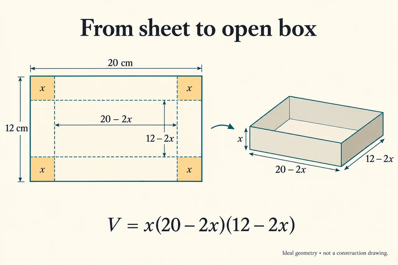
Image: illustration, not a documentary photograph. Ideal sheet and corner-cut schematic; shaded corners are removed, not folded into the box. Not a calibrated construction or strength drawing. · Original generated project artwork; no source textbook or exam-board figures reused.

From gradients to decisions: stationary points and a box with limits

A derivative graph tells you about the original curve's gradients, not its heights. Where f′ is positive the function increases; where it is negative the function decreases. A zero derivative identifies a stationary point if that input belongs to a differentiable part of the function. It does not by itself identify a maximum or minimum. Adding a constant to f shifts every height without changing f′. Therefore a derivative graph alone cannot provide the original vertical position unless a value or other condition is supplied. When a diagram asks you to recover behaviour, separate the direction of change, the locations of stationary inputs and the additional information needed to locate the curve.

Return to f(x) = x³−3x, already used in the first-principles lesson. Its derivative is 3x²−3 = 3(x−1)(x+1). It is positive for x < −1, negative for −1 < x < 1, and positive for x > 1. At −1 the gradient changes from positive to negative, so the point is a local maximum; its height is f(−1) = 2. At 1 the gradient changes from negative to positive, giving a local minimum with height −2. This complete sign argument connects an algebraic solution to actual behaviour on neighbouring intervals. Solving f′ = 0 without testing the intervals would leave the classification unfinished.

The second derivative measures how the first derivative changes. For this cubic, f″(x) = 6x. The curve is concave down for negative x and concave up for positive x; its concavity changes at x = 0. Since f(0) = 0, that point is an inflection point, and it is not stationary because f′(0) = −3. At a stationary point, a strictly positive second derivative gives a local minimum and a strictly negative one gives a local maximum under the usual twice-differentiable conditions. A zero second derivative does not settle the question. For x³ at 0 there is a stationary inflection; for x⁴ at 0 there is a minimum. Their signs on neighbouring intervals explain why the same zero test can leave different outcomes.

A useful derivative-graph exercise changes the information rather than merely the coefficients. Suppose a derivative crosses the horizontal axis at a, stays negative until b, then becomes positive, and is positive just before a. The original function has a local maximum at a and a local minimum at b. You cannot read their heights from the derivative's axis. If the derivative instead touches zero but remains positive on both sides, the original function continues increasing and has no local extremum there. Whether that point is an inflection requires further concavity evidence. These distinctions keep stationary inputs, extrema, inflections and the graph's vertical intercept from being treated as interchangeable labels.

Optimisation adds a model and a feasible domain. Imagine a rectangular sheet 20 cm long and 12 cm wide. Cut a square of side x cm from every corner and fold the remaining sides up to make an open box. Its height is x, its base length is 20−2x and its base width is 12−2x. Its ideal geometric volume is V(x) = x(20−2x)(12−2x) cubic centimetres. A positive-height box with positive base dimensions requires 0 < x < 6. A root outside that interval is not a second possible design. This model ignores sheet thickness, folding losses, strength and manufacturing allowances; maximising it does not certify a practical package.

Expanding gives V(x) = 4x³−64x²+240x, so V′(x) = 12x²−128x+240. Solving V′ = 0 gives x = (16±2√19)/3. The smaller root is approximately 2.4274 cm and lies in the feasible interval. The larger root, approximately 8.2393 cm, does not. The derivative is positive before the smaller root and negative after it throughout the remainder of 0 < x < 6. The candidate is consequently the global maximum on that interval, not merely a stationary point identified by algebra. As x approaches either boundary the volume approaches zero. Those limiting values help compare the complete feasible domain even though its two endpoints are not positive-volume boxes.

At x = (16−2√19)/3 the volume is approximately 262.68 cm³. Reporting only the cut size would leave the question about capacity unanswered; reporting only a volume would leave the construction unspecified. Keep the exact root until evaluating the final quantity to avoid unnecessary rounding error. The second derivative 24x−128 is negative at this root and confirms the local classification, while the interval argument establishes the global result. The volume's units are cubic centimetres, the cut size's units are centimetres, and V′ has units of square centimetres. A gradient is not another volume and cannot be substituted for the result that is being optimised.

Now change a real constraint within the fictional model. If a cutting tool permits only 0 < x ≤ 2 cm, the previously optimal cut is unavailable. The derivative is positive throughout this shorter interval, so the maximum is its included upper boundary x = 2 cm, giving 256 cm³. There is no stationary point inside the permitted range. This example explains why “differentiate and set equal to zero” is a candidate-finding technique rather than a complete optimisation method. State what is being maximised, derive the model, establish the allowable inputs, test stationary candidates and applicable boundaries, then answer in context. If the constraint, objective or assumptions change, repeat those steps instead of recycling the earlier optimum.

Further answered graph check

Question: At an input c, a differentiable function has derivative zero and its derivative graph stays positive immediately to either side. Does that prove a maximum, minimum or inflection?

Answer: It proves a stationary input but neither a maximum nor minimum, because the function keeps increasing locally across c. It does not alone prove an inflection; further information about the sign of the second derivative or a change in concavity is required. Function values are still needed to locate the point vertically.

Worked example: Fully worked classification
Classify all stationary points and inflection points of f(x) = x³−3x. Explain what changes if the function is replaced by f(x)+100.

Fully worked optimisation
Find the ideal maximum-volume open box made by the stated 20 cm by 12 cm sheet method. Justify a global result on the feasible domain.

Fully worked classification
1. Differentiate: f′(x) = 3x²−3. Solve f′ = 0 to obtain x = −1 and x = 1, both allowed because the polynomial has every real input.
2. Factor the derivative as 3(x−1)(x+1). Its signs on the three intervals are positive, negative and positive. Thus −1 gives a local maximum and 1 a local minimum.

Fully worked classification
3. Evaluate the original function, not its derivative, for the coordinates: (−1,2) and (1,−2). Their zero gradients do not make their heights zero.
4. The second derivative is 6x. Its sign changes from negative to positive at 0, establishing an inflection at (0,0). Its first derivative there is −3, so this inflection is not stationary.

Fully worked classification
5. Adding 100 changes none of these derivative formulas, stationary inputs or classifications. It changes the heights to 102, 98 and 100 respectively. A derivative graph cannot distinguish these two vertical positions without another supplied value.

Fully worked optimisation
1. With four square corner cuts of side x, the box dimensions are x, 20−2x and 12−2x cm. Positivity gives 0 < x < 6. Record this domain before solving a derivative equation.
2. Multiply the dimensions: V = 4x³−64x²+240x cm³. Differentiate: V′ = 12x²−128x+240, and divide the stationary equation by 4 to obtain 3x²−32x+60 = 0.

Fully worked optimisation
3. The quadratic formula gives x = (16±2√19)/3. Only (16−2√19)/3 lies in 0 < x < 6. Reject the other root for the geometric reason that a base dimension would not remain positive.
4. The derivative is positive before the allowed root and negative afterwards up to 6. The volume therefore rises to that candidate and falls after it over the entire feasible interval. Both boundary limits are zero, so no other feasible input has a larger volume.

Fully worked optimisation
5. Substitute the exact cut into the volume formula before rounding: x ≈ 2.4274 cm gives V ≈ 262.68 cm³. State both quantities and retain the ideal-sheet assumptions; this calculation does not predict material strength or available usable space with thick walls.

Answer: Fully worked classification
Local maximum (−1,2), local minimum (1,−2), nonstationary inflection (0,0). A constant vertical shift preserves the derivative information and changes all corresponding heights by that constant.

Fully worked optimisation
Cut x = (16−2√19)/3 cm, approximately 2.4274 cm, giving an ideal maximum volume of approximately 262.68 cm³.

Check your understanding: The same fictional sheet is processed by a tool allowing only 0 < x ≤ 2 cm. A learner recommends the earlier 2.4274 cm cut because it solves V′ = 0. Find the permitted optimum and assess that reasoning.

Answer: The earlier cut is outside the new domain and cannot be selected. On 0 < x ≤ 2 the derivative remains positive because this whole interval lies before its first zero at about 2.4274. Volume therefore increases throughout the permitted domain, so the included boundary x = 2 cm gives its maximum. The dimensions are 2 cm, 16 cm and 8 cm, and the volume is 2×16×8 = 256 cm³. The limiting volume as x tends to zero is zero. The answer is a boundary optimum with no permitted stationary point; the derivative method still applies when its candidate list is completed with constraints and boundaries. The result remains an ideal geometric account rather than a tested manufactured box.

Why: Now change a real constraint within the fictional model. If a cutting tool permits only 0 < x ≤ 2 cm, the previously optimal cut is unavailable. The derivative is positive throughout this shorter interval, so the maximum is its included upper boundary x = 2 cm, giving 256 cm³. There is no stationary point inside the permitted range. This example explains why “differentiate and set equal to zero” is a candidate-finding technique rather than a complete optimisation method. State what is being maximised, derive the model, establish the allowable inputs, test stationary candidates and applicable boundaries, then answer in context. If the constraint, objective or assumptions change, repeat those steps instead of recycling the earlier optimum.