Reading a curve as a graph of gradients
By UK A Level Mathematics · independent study · myAudience
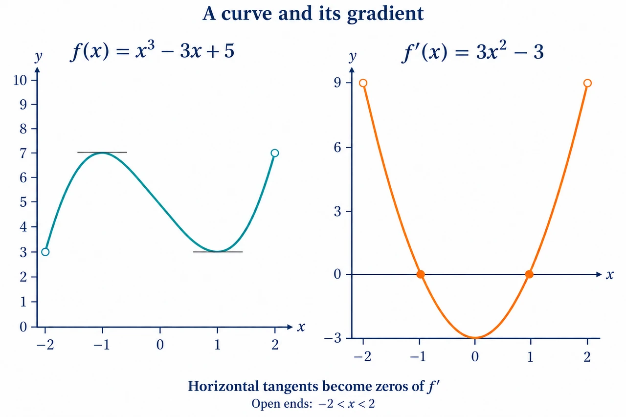
Image: illustration, not a documentary photograph. Each panel retains the same labelled input scale. The vertical rulers at the left panel boundaries are output scales, not x=0 axes. Rendered curves are schematic; use the formula and labelled coordinates for exact values. Open endpoints exclude −2 and2. · Original project illustration; rendered schematic teaching aid, not a calibrated measurement or exam-board figure.
Reading a curve as a graph of gradients
A derivative graph answers a different question from the original curve. At an input x, the height of f is the output of the function; the height of f′ is the slope of the tangent to that curve. Start by imagining a tiny straightedge resting against the curve. A tangent rising to the right supplies a positive derivative, a falling tangent a negative derivative, and a horizontal tangent a zero derivative. Whether the original curve lies above or below its horizontal axis is irrelevant to this sign. A high point on the page can have negative gradient, and a point below the axis can have positive gradient. Read the direction of the tangent, rather than copying the outline of the curve.
Keep the horizontal input scale unchanged when moving from f to f′. A horizontal tangent at x=2 places a zero of the derivative at input 2; it does not move the zero to the original curve's output value. The vertical scale changes meaning. If each horizontal grid square represents two input units while each vertical square represents three output units, a tangent rising one vertical square over two horizontal squares has gradient3/4, not1/2. Draw a sufficiently large tangent triangle and use differences in labelled coordinates. A small triangle magnifies drawing uncertainty. A schematic unscaled curve supports a qualitative sketch but cannot justify exact numerical derivative heights.
As you move along a smooth curve, compare neighbouring tangent slopes. If the curve is becoming more steeply positive, the derivative graph rises. If a curve is still decreasing but becoming less steeply negative, the derivative also rises, toward zero. This distinction separates the sign of f′ from whether f′ is increasing. A valley in f with negative-to-positive slopes becomes an axis crossing of f′. A horizontal tangent without a change of slope sign can become a touch of the derivative axis. Do not invent a maximum or minimum of f merely because its derivative is zero.
A smooth curve that changes from bending downward to bending upward has tangent slopes that first decrease and then increase. Where this transition occurs, its derivative can have a local minimum. The reverse bending transition can produce a local maximum of the derivative. These are useful connections, not a licence to read exact curvature from a rough illustration. A derivative's local extremum is not the same object as an extremum of the original function. Use the actual tangent pattern and the differentiability assumptions supplied. Zero second derivative alone does not prove an inflection.
A sharp corner needs a different symbol from a stationary point. For f(x)=|x|, the tangent slope is−1 on the left of 0 and+1 on the right, but the derivative does not exist at 0. The derivative sketch consists of two horizontal parts with open circles at their missing endpoints; putting a filled point at 0 would invent a derivative. A jump in f prevents a derivative there too. A vertical tangent can have no finite derivative: for the real cube-root curve, the difference quotient at 0 grows without bound positively. It has no ordinary real-valued derivative at that input. Mark a missing input or appropriate limiting behaviour; do not draw a finite connecting line just to make the derivative continuous.
Known straight sections provide unusually strong evidence. A horizontal segment has zero derivative at its interior inputs, while a straight segment of constant nonzero slope has a constant derivative there. At joins, inspect the two one-sided slopes rather than extending these conclusions automatically. At the boundary of a restricted domain, the usual two-sided derivative need not be defined; endpoint conventions or one-sided derivatives must be explicitly stated. A graph task on an open interval should therefore keep the corresponding derivative endpoints open. An asymptote of f need not be an asymptote of f′ of the same kind or sign.
Adding a constant to f moves the curve vertically without changing any tangent slope. Multiplying its outputs by a constant multiplies every derivative height by that constant. Replacing x by 2x compresses the input pattern horizontally and adds another factor 2 to the derivative: if g(x)=3f(2x)+7, then g′(x)=6f′(2x). A derivative point(a,b) therefore becomes(a/2,6b), on the transformed domain. The+7 contributes nothing to the derivative. Treat the coordinate transformation and the slope scaling as two separate operations, so a graph sketch does not miss the chain factor.
Source and scope boundaries
Official scope source: Pearson Edexcel 9MA0 Issue 4 February 2020, Pure 7.1, PDF page 26 in 1-based numbering (web P25), printed page22. Freshly checked 2026-10-05: https://qualifications.pearson.com/content/dam/pdf/A%20Level/Mathematics/2017/specification-and-sample-assesment/a-level-l3-mathematics-specification-issue4.pdf. This source supplies the assessed skill and the importance of axes/scales. All teaching, examples, numbers and answers above are original; no Pearson assessment task or mark scheme is reproduced. This lesson does not establish whole-qualification coverage or assessed mastery. The schematic illustration has been visually checked; its 160-pixel version is a recognition preview, not a substitute for the formulas and coordinates. Use the supplied formulas and coordinates to check the schematic graph and open endpoints; rendering appearance alone is not mathematical evidence.
A complete answer states what is known and what is estimated. Mark inputs with horizontal tangents, signs between them, increasing or decreasing derivative sections, any constant-slope intervals, exclusions, and numerical heights supported by actual tangent measurements. Then draw a curve consistent with all the evidence. Do not claim that finitely many slope measurements determine a unique formula or that the derivative graph can recover the original vertical position. In a position–time context, derivative units are length/time; for a velocity–time curve they are length/time². A negative acceleration describes a falling signed velocity, which is not automatically a falling speed when the velocity is negative.
Image caption: Each panel retains the same labelled input scale. The vertical rulers at the left panel boundaries are output scales, not x=0 axes. Rendered curves are schematic; use the formula and labelled coordinates for exact values. Open endpoints exclude −2 and2.
Worked example: A smooth curve on−2<x<2 has tangent slopes9 at −2 by right-limit,0 at −1,−3 at 0,0 at 1 and9 at 2 by left-limit. It rises for−2<x<−1, falls for−1<x<1 and rises for1<x<2. Its tangent slopes decrease up to 0 and increase after0. Sketch f′ with correct signs and exclusions. Each horizontal grid square of the supplied curve represents2 input units and each vertical square represents3 output units; explain the slope of a tangent that falls2 vertical squares while running1 horizontal square. Finally verify the sketch using f(x)=x³−3x+5, without pretending that the given measurements alone identified that formula.
First place open limiting points(−2,9) and(2,9), and actual zeros(−1,0),(1,0). Place(0,−3). The derivative is positive on(−2,−1) and(1,2), negative on(−1,1). Its decreasing-then-increasing evidence gives a minimum at(0,−3); join the marked values with a smooth U-shaped curve consistent with these facts. The original curve's outputs do not become derivative heights. The tangent triangle has output change−6 and input change2, so its slope is−3. Counting squares alone as−2 would ignore the units. Independently differentiate the supplied formula to obtain f′(x)=3x²−3; it reproduces every measured value and sign. Its graph is the specified part of a parabola. The+5 is undetectable in the derivative. The data could also have arisen from other functions; formula verification is conditional on the additional supplied formula, not a proof of uniqueness.
Worked model 2: zero gradient without a turning point
Task. A curve has formula h(x)=x³ on the whole real line. Sketch its gradient function using tangent behaviour, verify algebraically, and compare with a second curve k(x)=|x|. Explain why treating both curves as having derivative zero at 0 is wrong.
Reasoning. The cubic rises on both sides of 0 but flattens near 0. Its slopes are positive for nonzero inputs and0 at the origin, so the derivative touches its axis rather than crossing it. Differentiation gives h′(x)=3x², a nonnegative parabola. The original cubic has no local maximum or minimum at 0; its horizontal tangent occurs at a stationary inflection. For k, the left straight ray has slope −1 and the right ray+1. At0 the difference quotient is |u|/u, approaching different one-sided values. No common limit exists, so k′(0) does not exist. Draw y=−1 for x<0 and y=1 for x>0, with open circles at the two points over 0 and no filled point joining them.
Answer. A zero derivative is a genuine horizontal tangent at an input where the derivative exists. A corner is a failure of differentiability, even when the function itself is continuous. These graph features require different derivative sketches and different explanations.
Unfamiliar transfer: a compressed curve and a reversed vertical scale
Question. On(−2,2), let f(x)=x³−3x+5 and set q(x)=−2f(3x)+4. State q's domain, derivative, zeros and signs, and the coordinate transformation from f′ to q′. Does q′(0)>0 prove q(0)>0?
Complete answer. The domain is−2/3<x<2/3. By the chain rule q′(x)=−6f′(3x)=18−162x². The derivative zeros are x=−1/3 and x=1/3. It is positive between those roots and negative on(−2/3,−1/3) and(1/3,2/3). The derivative point(a,b) transforms to(a/3,−6b). In particular(0,−3) becomes(0,18), a derivative maximum; the limiting points(±2,9) become open limiting points(±2/3,−54). Although q′(0)=18>0, q(0)=−2·5+4=−6<0. The original height and its tangent slope have different meanings. The constant 4 does not affect q′.
Answer: On the open interval(−2,2), draw y=3x²−3 if the formula is supplied; otherwise label the consistent sketch as qualitative between the measured tangent values. Mark the two endpoint limits with open circles. The slope of the measured tangent is−3 output units per input unit. Original local extrema at −1 and1 become derivative zeros, whereas the derivative minimum occurs at 0.
Check your understanding: A signed velocity graph lies below its axis and slopes downward throughout a time interval. A learner concludes that the object is slowing down because its acceleration is negative. Evaluate the claim and state the derivative units when velocity is measured in m/s and time in seconds.
Answer: The derivative of signed velocity is negative acceleration with units m/s². Because velocity is negative and becoming more negative, its magnitude, and hence speed, increases on the interval. The object is speeding up in the negative direction. The claim confuses a decreasing signed value with a decreasing magnitude. If the curve instead showed positive velocity decreasing while staying positive, the same negative acceleration would mean slowing down. Any point at which velocity changes sign needs its own local speed analysis.
Why: Analyse two different graph features before interpreting the motion: height determines the sign of velocity, while local slope determines acceleration. In the below-axis interval the speed is −v, so its derivative is −a. This sign conversion is the decisive step; a downward slope alone cannot classify speeding up or slowing down. Dividing a velocity change by a time change also establishes the acceleration units. The reasoning applies only within the stated negative-velocity interval, not automatically across a zero crossing.