Recover a changing quantity from its rate
By UK A Level Mathematics · independent study · myAudience
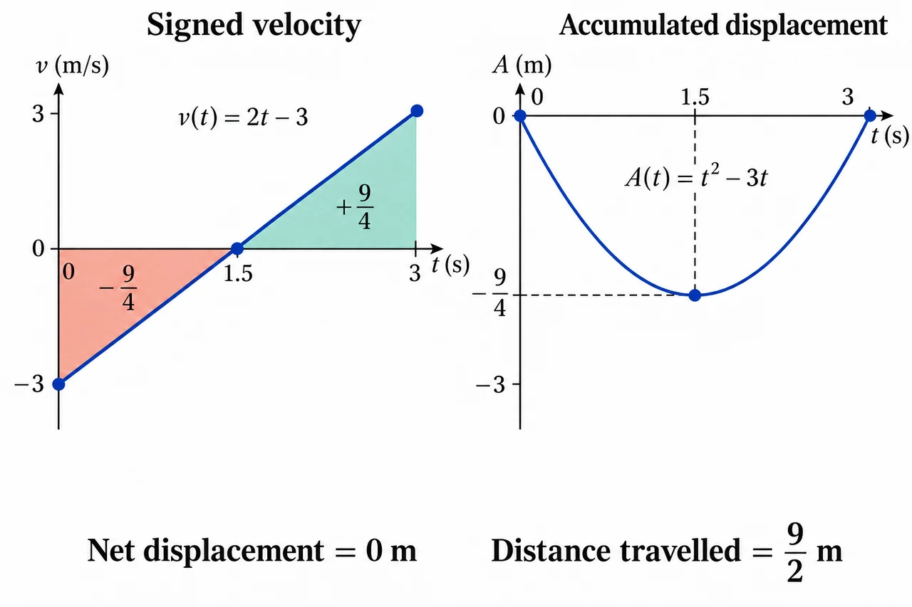
Image: illustration, not a documentary photograph. The panels share the same time scale but use different output units and scales. Velocity is v(t)=2t−3 m/s; accumulated displacement is A(t)=t²−3t m relative to the starting position. The negative and positive signed contributions are −9/4 m and +9/4 m. They cancel to zero displacement while distance is 9/2 m. The rendered lines and shading are schematic; formulas and labelled coordinates are authoritative. A 160-pixel preview supports recognition, not reading every label. · Original project scientific illustration; schematic teaching aid, not a calibrated measurement or exam-board figure.
Recover a changing quantity from its rate
A rate describes how a quantity is changing; it does not tell us the quantity's starting value. If a curve has gradient 3x², then both x³ and x³+40 produce that rate. Integrating an expression asks for a family of functions whose derivative is that expression. The notation ∫f(x) dx means an indefinite integral: an antiderivative plus an arbitrary constant, not a number obtained by substituting endpoints. By contrast, ∫ₐᵇf(x) dx describes accumulated signed change over a specified interval. Keep these two questions separate: “Which functions have this rate?” and “How much change occurred between these inputs?” An initial measurement answers the first question's remaining uncertainty; it is unnecessary for finding the second question's net change.
Define A(x)=∫ₐˣf(t) dt for a continuous rate f on an interval containing a and x. The t is a dummy variable inside the integral; x controls its upper endpoint. Between x and x+h, accumulation changes by ∫ₓˣ⁺ʰf(t) dt. Dividing that change by h gives the average rate over this short interval. Continuity means that every nearby f(t) becomes close to f(x), so this average tends to f(x) as h tends to zero. This works from either direction: when h is negative, reversing the integral's bounds and dividing by negative h leaves the ordinary average over the same small interval. Thus A′(x)=f(x) at interior points. This reasoning assumes the ordinary definite integral and its interval-addition and bounding properties; it is a local continuity argument, not a claim that every arbitrary function has an antiderivative.
An independently known antiderivative F also satisfies F′=f. Therefore F−A has zero derivative wherever both are defined on the interval. The mean value theorem implies that a differentiable function with zero derivative is constant on a connected interval. Since A(a)=0, that constant is F(a), and A(b)=F(b)−F(a). This is the bridge from accumulating a rate to evaluating its antiderivative at endpoints. The order matters: upper endpoint first, lower endpoint second. Reversing the bounds reverses the sign. The constant C cancels in a definite integral because the same constant belongs to both endpoint evaluations on the same interval. It cannot be cancelled across disconnected branches merely because two expressions look similar.
The integration power rule follows by checking a derivative. For n≠−1, differentiating xⁿ⁺¹/(n+1) gives xⁿ wherever the real powers involved are differentiable. Hence ∫xⁿ dx=xⁿ⁺¹/(n+1)+C on an appropriate interval. The exponent increases by one and the coefficient divides by that new exponent. Constant multiples and sums can be integrated term by term because differentiation is linear. The excluded case n=−1 would divide by zero; its antiderivative belongs to a logarithmic topic, not this power rule. Rational powers require their real domains to be checked. For example, x¹ᐟ² is real for x≥0, but formulas containing x⁻² require x≠0. A formula derived on x>0 does not automatically establish behavior through zero or on a different real branch.
To recover a particular curve, first find the full antiderivative family, then substitute the given point into the function rather than its derivative. A statement F(1)=5 constrains F, whereas F′(1)=5 constrains the rate. They are different data. Afterwards differentiate the proposed F to check the entire original rate and evaluate the initial condition again. Both checks matter: a correct derivative with the wrong constant misses the given point; a curve through the right point with the wrong derivative misses the required rates elsewhere. If the model uses metres and seconds, a velocity integrated against seconds has units of metres. Adding an arbitrary dimensionless number to a position formula is not a physically coherent interpretation of C; the integration constant has the quantity's units.
A definite integral tracks sign. Negative rate can undo an earlier positive change, so a zero integral need not mean that nothing happened. For a rate that changes sign, split the interval at its zeros before asking for a total unsigned amount. For a velocity v, signed displacement is ∫v dt but distance is ∫|v| dt. For a mathematical graph, signed area and total geometric area follow the same distinction. Integrating the absolute value of a rate usually means replacing it by the appropriate piecewise formulas; it does not mean taking the absolute value of the final signed integral. Cancellation takes place before that final absolute value and would conceal any movement in opposite directions.
Continuity is a sufficient hypothesis for the form of the fundamental theorem used here. Its absence means that this justification must be reconsidered, not that every conclusion is automatically false. For a step rate r(t)=−1 when t<1 and r(t)=1 when t≥1, accumulation from 0 is A(x)=−x on 0≤x≤1 and A(x)=x−2 on x≥1. A is continuous at 1, but its left slope is −1 and its right slope is 1, so A′(1) does not exist. Changing just the assigned value r(1) cannot fix those different one-sided slopes. Conversely, a single removable discontinuity can leave an accumulation function differentiable there while its derivative differs from the rate's arbitrarily reassigned point value. Check the actual hypotheses and the actual conclusion; do not reduce the theorem to a slogan.
A variable endpoint adds a second rate of change. If B(u)=∫ₐᵘf(t) dt and H(x)=B(g(x)), then H′(x)=f(g(x))g′(x) where continuity, differentiability and interval-domain conditions hold. The factor g′ accounts for how rapidly the upper endpoint moves; omitting it is a chain-rule error. A disconnected domain brings a different limitation: a derivative fixes an integration constant only within a connected component. For F′(x)=−1/x² on x≠0, F=1/x+C₊ on x>0 and F=1/x+C₋ on x<0. One measurement at x=1 fixes C₊ but says nothing about C₋. An ordinary finite-interval integral across zero cannot be evaluated using the continuous-interval theorem. This lesson opens integration reasoning; it does not complete integration techniques, improper integrals, differential-equation modelling or assessed qualification coverage.
Sources, rights and open scope
Official scope: Pearson Edexcel 9MA0 Issue 4 February 2020, Pure 8.1/8.2, PDF page28 (1-based), printed24; sign-aware definite evaluation touches8.3 on PDF29/printed25. Existing source records8-1-01/02 and8-2-01 are AS-and-A-Level;8-3-01 has the same mode. Only existing source requirements are bound; assessment stays open. Official wording is retained privately as source evidence, not copied as an exam task or mark scheme.
Verification reference: OpenStax Calculus Volume1 5.3, theorem5.4 continuous-rate accumulation and theorem5.5 evaluation. Standard theorems are expressed independently; every numeric task and worked answer above is original. No publisher diagram, worked exercise or text is reused as a deliverable. The full proof here relies on standard integration and mean-value facts named explicitly. Whole integration, independent assessment, AS readiness and full qualification remain open. The selected schematic illustration and its 1280-, 640- and 160-pixel variants have been visually checked; formulas and labelled coordinates are authoritative, and the 160-pixel preview supports recognition.
Image: illustration, not a documentary photograph. The panels share the same time scale but use different output units and scales. Velocity is v(t)=2t−3 m/s; accumulated displacement is A(t)=t²−3t m relative to the starting position. The negative and positive signed contributions are −9/4 m and +9/4 m. They cancel to zero displacement while distance is 9/2 m. The rendered lines and shading are schematic; formulas and labelled coordinates are authoritative. A 160-pixel preview supports recognition, not reading every label.
Worked example: Worked model 1 — A gradient and a point
Question: F′(x)=3x²−4x+2 for all real x and F(1)=5. Find F(x), calculate ∫₀³F′(x) dx and explain why the initial measurement is irrelevant to that integral.
Worked model 2 — Signed change and total movement
Question: A particle moves along a straight line with idealized velocity v(t)=2t−3 metres per second for 0≤t≤3 seconds. Find its displacement, its distance travelled and the time when its position is smallest. Explain what data are missing if its final position is requested.
Worked model 3 — Powers, restrictions and an initial value
Question: G′(x)=4√x−3/x² on x>0 and G(1)=2. Recover G and verify the result.
Changed task 1 — An endpoint that moves twice as fast
Question: H(x)=∫₁²ˣ(t²+1) dt for every real x, including x<1/2 when the upper bound is smaller than the lower. Find an exact formula for H, find H′(x), and evaluate H(0). Explain the tempting wrong answer 4x²+1.
Changed task 2 — One point cannot connect two branches
Question: F′(x)=−1/x² on x≠0 and F(1)=7. A student claims F(−1)=5 because F(x)=1/x+6 for all x≠0. Is the conclusion forced? Can ∫₋₁¹−1/x² dx be found by subtracting those endpoints?
Integrating each term gives F(x)=x³−2x²+2x+C. Substituting x=1 into the function gives 1−2+2+C=5, hence C=4. The required curve is F(x)=x³−2x²+2x+4. Differentiating recovers 3x²−4x+2; evaluating F(1) recovers 5, so both checks pass. For the definite integral use F(3)−F(0)=19−4=15. Any choice of C gives the same difference because it appears at both endpoints and cancels. An initial measurement chooses the vertical position of the curve; it cannot change its accumulated rate over this fixed interval. The rate is positive everywhere: completing the square gives 3(x−2/3)²+2/3. Thus this integral is also the geometric area between the rate graph and its horizontal axis, but that agreement depends on the sign check.
An antiderivative of v is P(t)=t²−3t, so displacement is P(3)−P(0)=0 metres. The velocity is negative before t=3/2, zero at t=3/2 and positive afterwards. At that turning time P(3/2)=−9/4. The first part contributes signed change −9/4 metres and the second contributes +9/4 metres. Distance is their unsigned sum, 9/2 metres, not |0|. Position decreases and then increases, so it is smallest at t=3/2 seconds. Writing position as s(t)=s(0)+t²−3t makes the missing initial position explicit: s(3)=s(0). The particle returns to its starting position, but the model supplies no absolute location. Constant acceleration 2 metres per second squared is an ideal model assumption; no claim is made about a particular vehicle or measured journey.
Write the derivative as 4x¹ᐟ²−3x⁻². The power rule gives G(x)=(8/3)x³ᐟ²+3x⁻¹+C. Evaluating at 1 gives 8/3+3+C=2, so C=−11/3. Therefore G(x)=(8/3)x³ᐟ²+3/x−11/3, x>0. The derivative is 4x¹ᐟ²−3x⁻², and G(1)=8/3+9/3−11/3=2. The domain stays x>0; the reciprocal term prevents continuation through zero, and the prescribed square root is not real for negative x. Nothing in the calculation permits dropping this restriction.
An antiderivative is t³/3+t, so H(x)=8x³/3+2x−4/3 and H(0)=−4/3. Differentiation gives H′(x)=8x²+2. The theorem gives the same result: the integrand evaluated at 2x is 4x²+1, and the upper endpoint has derivative 2, producing 2(4x²+1). The wrong answer omits the endpoint's motion. The polynomial integrand is continuous on every real interval, and the reversed-bound definition handles x<1/2 without changing the formula. The negative value at zero is an orientation effect, not a negative geometric area.
No. On x>0 the condition gives C₊=6, but on x<0 the independent constant C₋ is unrestricted. Therefore F(−1)=−1+C₋ may take any real value; 5 is one possible choice, not a consequence of the data. The zero-derivative uniqueness argument only connects points in the same interval. The integral crosses a pole where the rate is undefined and is not the ordinary continuous finite-interval integral used in this lesson. If it is instead interpreted as an improper integral, the two sides must be evaluated separately. On [−1,−ε], the integral is −1/ε+1, and on [ε,1] it is 1−1/ε; each tends to −∞ as ε tends to zero. It has no finite value. Subtracting 1−(−1)=2 ignores the singularity and applies the theorem outside its hypotheses.
Answer: The required curve is F(x)=x³−2x²+2x+4. For the definite integral use F(3)−F(0)=19−4=15. Distance is their unsigned sum, 9/2 metres, not |0|. Therefore G(x)=(8/3)x³ᐟ²+3/x−11/3, x>0. Differentiation gives H′(x)=8x²+2. Therefore F(−1)=−1+C₋ may take any real value; 5 is one possible choice, not a consequence of the data.
Check your understanding: Question: For the velocity in worked model 2, a student says “The integral is zero, so its speed was zero throughout.” Give the exact counterevidence and the smallest method change needed to calculate distance.
Answer: At t=0, v=−3 metres per second, so the speed is 3 metres per second; at t=3, it is also 3. Nonzero rates occur throughout except at t=3/2. The zero displacement results from two opposite signed changes, not zero speed. Split the interval at 3/2 and integrate −v on the first part and v on the second, producing 9/4+9/4=9/2 metres. This changes the integrand to |v| before adding contributions; taking the absolute value after the signed integral cannot recover the cancelled movement.
Why: The claim confuses cancellation across an interval with the behavior at individual times. A signed integral combines oriented contributions; it cannot show that each rate was zero. Distinguish the rate graph from an accumulated position graph, then locate each change of direction before interpreting a total. The units also provide a check: speed is measured in metres per second, while the time integral of speed is measured in metres. An absolute value applied to an already accumulated displacement answers a different question from adding nonnegative travelled lengths.